Building a Visceral Understanding of Quantum Phenomena

A great childhood memory that I have comes from first playing “The Incredible Machine” on PC in the early 90’s. For those not in the know, this is a physics-based puzzle game about building Rube Goldberg style contraptions to achieve given tasks. What made this game a standout for me was the freedom that it granted players. In many levels you were given a disparate set of components (e.g. strings, pulleys, rubber bands, scissors, conveyor belts, Pokie the Cat…) and it was entirely up to you to “MacGuyver” your way to some kind of solution (incidentally, my favorite TV show from that time period). In other words, it was often a creative exercise in designing your own solution, rather than “connecting the dots” to find a single intended solution. Growing up with games like this undoubtedly had significant influence in directing me to my profession as a research scientist: a job which is often about finding novel or creative solutions to a task given a limited set of tools.

From the late 90’s onwards puzzle games like “The Incredible Machine” largely went out of fashion as developers focused more on 3D games that exploited that latest hardware advances. However, this genre saw a resurgence in 2010’s spearheaded by developer “Zachtronics” who released a plethora of popular, and exceptionally challenging, logic and programming based puzzle games (some of my favorites include Opus Magnum and TIS-100). Zachtronics games similarly encouraged players to solve problems through creative designs, but also had the side-effect of helping players to develop and practice tangible programming skills (e.g. design patterns, control flow, optimization). This is a really great way to learn, I thought to myself.

So, fast-forward several years, while teaching undergraduate/graduate quantum courses at Georgia Tech I began thinking about whether it would be possible to incorporate quantum mechanics (and specifically quantum circuits) into a Zachtronics-style puzzle game. My thinking was that such a game might provide an opportunity for students to experiment with quantum through a hands-on approach, one that encouraged creativity and self-directed exploration. I was also hoping that representing quantum processes through a visual language that emphasized geometry, rather than mathematical language, could help students develop intuition in this setting. These thoughts ultimately led to the development of The Qubit Factory. At its core, this is a quantum circuit simulator with a graphic interface (not too dissimilar to the Quirk quantum circuit simulator) but providing a structured sequence of challenges, many based on tasks of real-life importance to quantum computing, that players must construct circuits to solve.
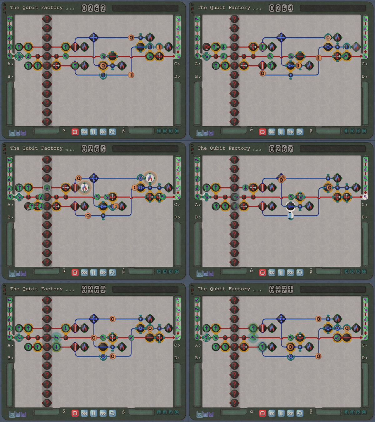
An example level of The Qubit Factory in action, showcasing a potential solution to a task involving quantum error correction. The column of “?” tiles represents a noisy channel that has a small chance of flipping any qubit that passes through. Players are challenged to send qubits from the input on the left to the output on the right while mitigating errors that occur due to this noisy channel. The solution shown here is based on a bit-flip code, although a more advanced strategy is required to earn a bonus star for the level!

Quantum Gamification and The Qubit Factory

My goal in designing The Qubit Factory was to provide an accurate simulation of quantum mechanics (although not necessarily a complete one), such that players could learn some authentic, working knowledge about quantum computers and how they differ from regular computers. However, I also wanted to make a game that was accessible to the layperson (i.e. without a prior knowledge of quantum mechanics or the underlying mathematical foundations like linear algebra). These goals, which are largely opposing one-another, are not easy to balance!

A key step in achieving this balance was to find a suitable visual depiction of quantum states and processes; here the Bloch sphere, which provides a simple geometric representation of qubit states, was ideal. However, it is also here that I made my first major compromise to the scope of the physics within the game by restricting the game state to real-valued wave-functions (which in turn implies that only gates which transform qubits within the X-Z plane can be allowed). I feel that this compromise was ultimately the correct choice: it greatly enhanced the visual clarity by allowing qubits to be represented as arrows on a flat disk rather than on a sphere, and similarly allowed the action of single-qubit gates to depicted clearly (i.e. as rotations and flips on the disk). Some purists may object to this limitation on grounds that it prevents universal quantum computation, but my counterpoint would be that there are still many interesting quantum tasks and algorithms that can be performed within this restricted scope. In a similar spirit, I decided to forgo the standard quantum circuit notation: instead I used stylized circuits to emphasize the geometric interpretation as demonstrated in the example below. This choice was made with the intention of allowing players to infer the action of gates from the visual design alone.

A quantum circuit in conventional notation versus the same circuit depicted in The Qubit Factory.

Okay, so while the Bloch sphere provides a nice way to represent (unentangled) single qubit states, we also need a way to represent entangled states of multiple qubits. Here I made use of some creative license to show entangled states as blinking through the basis states. I found this visualization to work well for conveying simple states such as the singlet state presented below, but players are also able to view the complete list of wave-function amplitudes if necessary.

\textrm{Singlet: }\left| \psi \right\rangle = \tfrac{1}{\sqrt{2}} \left( \left| \uparrow \downarrow \right\rangle - \left| \downarrow \uparrow \right\rangle \right)

A singlet state is created by entangling a pair of qubits via a CNOT gate.

Although the blinking effect is not a perfect solution for displaying superpositions, I think that it is useful in conveying key aspects like uncertainty and correlation. The animation below shows an example of the entangled wave-function collapsing when one of the qubits is measured.
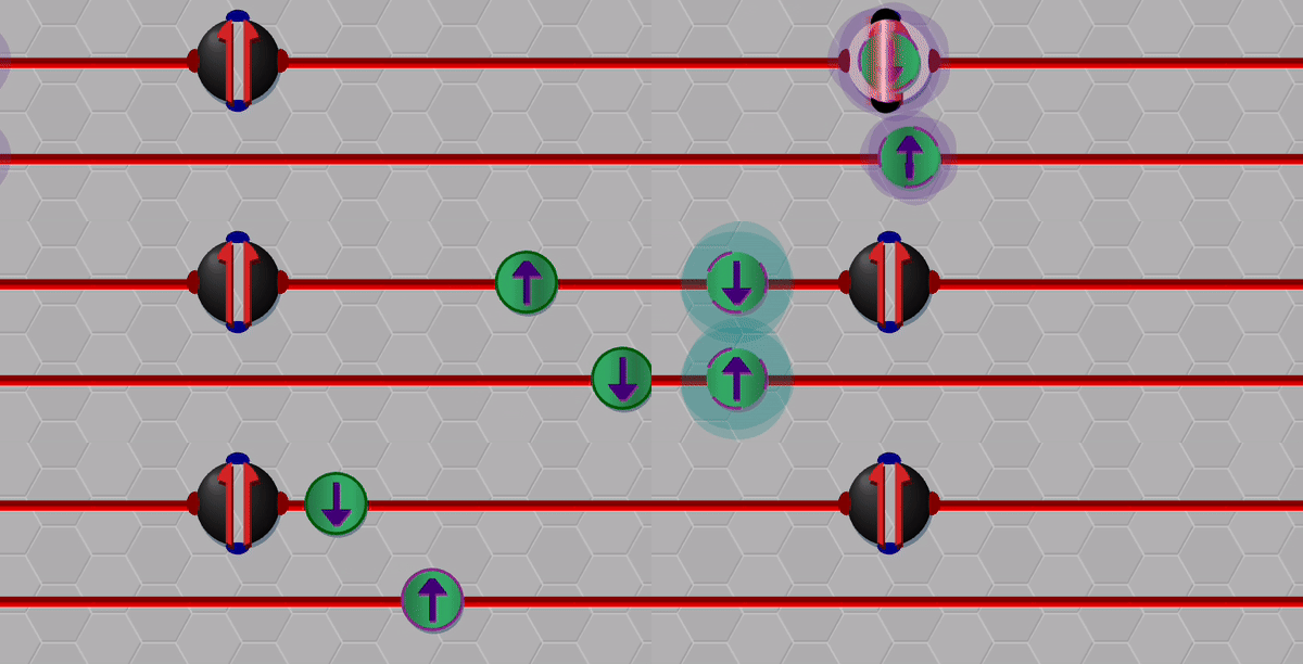
A single qubit from a singlet is measured. While each qubit has a 50/50 chance of giving ▲ or ▼ when measured individually, once one qubit is measured the other qubit collapses to the anti-aligned state.

So, thus far, I have described a quantum circuit simulator with some added visual cues and animations, but how can this be turned into a game? Here, I leaned heavily on the existing example of Zachtronic (and Zachtronic-like) games: each level in The Qubit Factory provides the player with some input bits/qubits and requires the player to perform some logical task in order to produce a set of desired outputs. Some of the levels within the game are highly structured, similar to textbook exercises. They aim to teach a specific concept and may only have a narrow set of potential solutions. An example of such a structured level is the first quantum level (lvl QI.A) which tasks the player with inverting a sequence of single qubit gates. Of course, this problem would be trivial to those of you already familiar with quantum mechanics: you could use the linear algebra result (AB)^\dag = B^\dag A^\dag together with the knowledge that quantum gates are unitary, so the Hermitian conjugate of each gate doubles as its inverse. But what if you didn’t know quantum mechanics, or even linear algebra? Could this problem be solved through logical reasoning alone? This is where I think that the visuals really help; players should be able to infer several key points from geometry alone:

  • the inverse of a flip (or mirroring about some axis) is another equal flip.
  • the inverse of a rotation is an equal rotation in the opposite direction.
  • the last transformation done on each qubit should be the first transformation to be inverted.

So I think it is plausible that, even without prior knowledge in quantum mechanics or linear algebra, a player could not only solve the level but also grasp some important concepts (i.e. that quantum gates are invertible and that the order in which they are applied matters).

An early level challenges the player to invert the action of the 3 gates on the left. A solution is given on the right, formed by composing the inverse of each gate in reverse order.

Many of the levels in The Qubit Factory are also designed to be open-ended. Such levels, which often begin with a blank factory, have no single intended solution. The player is instead expected to use experimentation and creativity to design their own solution; this is the setting where I feel that the “game” format really shines. An example of an open-ended level is QIII.E, which gives the player 4 copies of a single qubit state \left| \psi \right\rangle, guaranteed to be either the +Z or +X eigenstate, and tasks the player to determine which state they have been given. Those familiar with quantum computing will recognize this as a relatively simple problem in state tomography. There are many viable strategies that could be employed to solve this task (and I am not even sure of the optimal one myself). However, by circumventing the need for a mathematical calculation, the Qubit Factory allows players to easily and quickly explore different approaches. Hopefully this could allow players to find effective strategies through trial-and-error, gaining some understanding of state tomography (and why it is challenging) in the process.
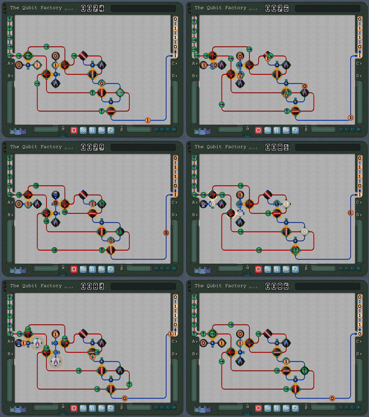
An example of a level in action! This level challenges the player to construct a circuit that can identify an unknown qubit state given several identical copies; a task in state tomography. The solution shown here uses a cascaded sequence of measurements, where the result of one measurement is used to control the axis of a subsequent measurement.

The Qubit Factory begins with levels covering the basics of qubits, gates and measurements. It later progresses to more advanced concepts like superpositions, basis changes and entangled states. Finally it culminates with levels based on introductory quantum protocols and algorithms (including quantum error correction, state tomography, super-dense coding, quantum repeaters, entanglement distillation and more). Even if you are familiar with the aforementioned material you should still be in for a substantial challenge, so please check it out if that sounds like your thing!

The Potential of Quantum Games

I believe that interactive games have great potential to provide new opportunities for people to better understand the quantum realm (a position shared by the IQIM, members of which have developed several projects in this area). As young children, playing is how we discover the world around us and build intuition for the rules that govern it. This is perhaps a significant reason why quantum mechanics is often a challenge for new students to learn; we don’t have direct experience or intuition with the quantum world in the same way that we do with the classical world. A quote from John Preskill puts it very succinctly:

“Perhaps kids who grow up playing quantum games will acquire a visceral understanding of quantum phenomena that our generation lacks.”


The Qubit Factory can be played at www.qubitfactory.io

To thermalize, or not to thermalize, that is the question.

The Noncommuting-Charges World Tour (Part 3 of 4)

This is the third part of a four-part series covering the recent Perspective on noncommuting charges. I’ll post one part every ~5 weeks leading up to my PhD thesis defence. You can find Part 1 here and Part 2 here.

If Hamlet had been a system of noncommuting charges, his famous soliloquy may have gone like this…

To thermalize, or not to thermalize, that is the question:
Whether ’tis more natural for the system to suffer
The large entanglement of thermalizing dynamics,
Or to take arms against the ETH
And by opposing inhibit it. To die—to thermalize,
No more; and by thermalization to say we end
The dynamical symmetries and quantum scars
That complicate dynamics: ’tis a consummation
Devoutly to be wish’d. To die, to thermalize;
To thermalize, perchance to compute—ay, there’s the rub:
For in that thermalization our quantum information decoheres,
When our coherence has shuffled off this quantum coil,
Must give us pause—there’s the respect
That makes calamity of resisting thermalization.

Hamlet (the quantum steampunk edition)


In the original play, Hamlet grapples with the dilemma of whether to live or die. Noncommuting charges have a dilemma regarding whether they facilitate or impede thermalization. Among the five research opportunities highlighted in the Perspective article, resolving this debate is my favourite opportunity due to its potential implications for quantum technologies. A primary obstacle in developing scalable quantum computers is mitigating decoherence; here, thermalization plays a crucial role. If systems with noncommuting charges are shown to resist thermalization, they may contribute to quantum technologies that are more resistant to decoherence. Systems with noncommuting charges, such as spin systems and squeezed states of light, naturally occur in quantum computing models like quantum dots and optical approaches. This possibility is further supported by recent advances demonstrating that non-Abelian symmetric operations are universal for quantum computing (see references 1 and 2).

In this penultimate blog post of the series, I will review some results that argue both in favour of and against noncommuting charges hindering thermalization. This discussion includes content from Sections III, IV, and V of the Perspective article, along with a dash of some related works at the end—one I recently posted and another I recently found. The results I will review do not directly contradict one another because they arise from different setups. My final blog post will delve into the remaining parts of the Perspective article.

Playing Hamlet is like jury duty for actors–sooner or later, you’re getting the call (source).

Arguments for hindering thermalization

The first argument supporting the idea that noncommuting charges hinder thermalization is that they can reduce the production of thermodynamic entropy. In their study, Manzano, Parrondo, and Landi explore a collisional model involving two systems, each composed of numerous subsystems. In each “collision,” one subsystem from each system is randomly selected to “collide.” These subsystems undergo a unitary evolution during the collision and are subsequently returned to their original systems. The researchers derive a formula for the entropy production per collision within a certain regime (the linear-response regime). Notably, one term of this formula is negative if and only if the charges do not commute. Since thermodynamic entropy production is a hallmark of thermalization, this finding implies that systems with noncommuting charges may thermalize more slowly. Two other extensions support this result.

The second argument stems from an essential result in quantum computing. This result is that every algorithm you want to run on your quantum computer can be broken down into gates you run on one or two qubits (the building blocks of quantum computers). Marvian’s research reveals that this principle fails when dealing with charge-conserving unitaries. For instance, consider the charge as energy. Marvian’s results suggest that energy-preserving interactions between neighbouring qubits don’t suffice to construct all energy-preserving interactions across all qubits. The restrictions become more severe when dealing with noncommuting charges. Local interactions that preserve noncommuting charges impose stricter constraints on the system’s overall dynamics compared to commuting charges. These constraints could potentially reduce chaos, something that tends to lead to thermalization.

Adding to the evidence, we revisit the eigenstate thermalization hypothesis (ETH), which I discussed in my first post. The ETH essentially asserts that if an observable and Hamiltonian adhere to the ETH, the observable will thermalize. This means its expectation value stabilizes over time, aligning with the expectation value of the thermal state, albeit with some important corrections. Noncommuting charges cause all kinds of problems for the ETH, as detailed in these two posts by Nicole Yunger Halpern. Rather than reiterating Nicole’s succinct explanations, I’ll present the main takeaway: noncommuting charges undermine the ETH. This has led to the development of a non-Abelian version of the ETH by Murthy and collaborators. This new framework still predicts thermalization in many, but not all, cases. Under a reasonable physical assumption, the previously mentioned corrections to the ETH may be more substantial.

If this story ended here, I would have needed to reference a different Shakespearean work. Fortunately, the internal conflict inherent in noncommuting aligns well with Hamlet. Noncommuting charges appear to impede thermalization in various aspects, yet paradoxically, they also seem to promote it in others.

Arguments for promoting thermalization

Among the many factors accompanying the thermalization of quantum systems, entanglement is one of the most studied. Last year, I wrote a blog post explaining how my collaborators and I constructed analogous models that differ in whether their charges commute. One of the paper’s results was that the model with noncommuting charges had higher average entanglement entropy. As a result of that blog post, I was invited to CBC’s “Quirks & Quarks” Podcast to explain, on national radio, whether quantum entanglement can explain the extreme similarities we see in identical twins who are raised apart. Spoilers for the interview: it can’t, but wouldn’t it be grand if it could?

Following up on that work, my collaborators and I introduced noncommuting charges into monitored quantum circuits (MQCs)—quantum circuits with mid-circuit measurements. MQCs offer a practical framework for exploring how, for example, entanglement is affected by the interplay between unitary dynamics and measurements. MQCs with no charges or with commuting charges have a weakly entangled phase (“area-law” phase) when the measurements are done often enough, and a highly entangled phase (“volume-law” phase) otherwise. However, in MQCs with noncommuting charges, this weakly entangled phase never exists. In its place, there is a critical phase marked by long-range entanglement. This finding supports our earlier observation that noncommuting charges tend to increase entanglement.

I recently looked at a different angle to this thermalization puzzle. It’s well known that most quantum many-body systems thermalize; some don’t. In those that don’t, what effect do noncommuting charges have? One paper that answers this question is covered in the Perspective. Here, Potter and Vasseur study many-body localization (MBL). Imagine a chain of spins that are strongly interacting. We can add a disorder term, such as an external field whose magnitude varies across sites on this chain. If the disorder is sufficiently strong, the system “localizes.” This implies that if we measured the expectation value of some property of each qubit at some time, it would maintain that same value for a while. MBL is one type of behaviour that resists thermalization. Potter and Vasseur found that noncommuting charges destabilize MBL, thereby promoting thermalizing behaviour.

In addition to the papers discussed in our Perspective article, I want to highlight two other studies that study how systems can avoid thermalization. One mechanism is through the presence of “dynamical symmetries” (there are “spectrum-generating algebras” with a locality constraint). These are operators that act similarly to ladder operators for the Hamiltonian. For any observable that overlaps with these dynamical symmetries, the observable’s expectation value will continue to evolve over time and will not thermalize in accordance with the Eigenstate Thermalization Hypothesis (ETH). In my recent work, I demonstrate that noncommuting charges remove the non-thermalizing dynamics that emerge from dynamical symmetries.

Additionally, I came across a study by O’Dea, Burnell, Chandran, and Khemani, which proposes a method for constructing Hamiltonians that exhibit quantum scars. Quantum scars are unique eigenstates of the Hamiltonian that do not thermalize despite being surrounded by a spectrum of other eigenstates that do thermalize. Their approach involves creating a Hamiltonian with noncommuting charges and subsequently breaking the non-Abelian symmetry. When the symmetry is broken, quantum scars appear; however, if the non-Abelian symmetry were to be restored, the quantum scars vanish. These last three results suggest that noncommuting charges impede various types of non-thermalizing dynamics.

Unlike Hamlet, the narrative of noncommuting charges is still unfolding. I wish I could conclude with a dramatic finale akin to the duel between Hamlet and Laertes, Claudius’s poisoning, and the proclamation of a new heir to the Danish throne. However, that chapter is yet to be written. “To thermalize or not to thermalize?” We will just have to wait and see.

Noncommuting charges are much like Batman

The Noncommuting-Charges World Tour Part 2 of 4

This is the second part of a four-part series covering the recent Perspective on noncommuting charges. I’ll post one part every ~5 weeks leading up to my PhD thesis defence. You can find part 1 here.

Understanding a character’s origins enriches their narrative and motivates their actions. Take Batman as an example: without knowing his backstory, he appears merely as a billionaire who might achieve more by donating his wealth rather than masquerading as a bat to combat crime. However, with the context of his tragic past, Batman transforms into a symbol designed to instill fear in the hearts of criminals. Another example involves noncommuting charges. Without understanding their origins, the question “What happens when charges don’t commute?” might appear contrived or simply devised to occupy quantum information theorists and thermodynamicists. However, understanding the context of their emergence, we find that numerous established results unravel, for various reasons, in the face of noncommuting charges. In this light, noncommuting charges are much like Batman; their backstory adds to their intrigue and clarifies their motivation. Admittedly, noncommuting charges come with fewer costumes, outside the occasional steampunk top hat my advisor Nicole Yunger Halpern might sport.

Growing up, television was my constant companion. Of all the shows I’d get lost in, ‘Batman: The Animated Series’ stands the test of time. I highly recommend giving it a watch.

In the early works I’m about to discuss, a common thread emerges: the initial breakdown of some well-understood derivations and the effort to establish a new derivation that accommodates noncommuting charges. These findings will illuminate, yet not fully capture, the multitude of results predicated on the assumption that charges commute. Removing this assumption is akin to pulling a piece from a Jenga tower, triggering a cascade of other results. Critics might argue, “If you’re merely rederiving known results, this field seems uninteresting.” However, the reality is far more compelling. As researchers diligently worked to reconstruct this theoretical framework, they have continually uncovered ways in which noncommuting charges might pave the way for new physics. That said, the exploration of these novel phenomena will be the subject of my next post, where we delve into the emerging physics. So, I invite you to stay tuned. Back to the history…

E.T. Jaynes’s 1957 formalization of the maximum entropy principle has a blink-and-you’ll-miss-it reference to noncommuting charges. Consider a quantum system, similar to the box discussed in Part 1, where our understanding of the system’s state is limited to the expectation values of certain observables. Our aim is to deduce a probability distribution for the system’s potential pure states that accurately reflects our knowledge without making unjustified assumptions. According to the maximum entropy principle, this objective is met by maximizing the entropy of the distribution, which serve as a measure of uncertainty. This resulting state is known as the generalized Gibbs ensemble. Jaynes noted that this reasoning, based on information theory for the generalized Gibbs ensemble, remains valid even when our knowledge is restricted to the expectation values of noncommuting charges. However, later scholars have highlighted that physically substantiating the generalized Gibbs ensemble becomes significantly more challenging when the charges do not commute. Due to this and other reasons, when the system’s charges do not commute, the generalized Gibbs ensemble is specifically referred to as the non-Abelian thermal state (NATS).

For approximately 60 years, discussions about noncommuting charges remain dormant, outside a few mentions here and there. This changed when two studies highlighted how noncommuting charges break commonplace thermodynamics derivations. The first of these, conducted by Matteo Lostaglio as part of his 2014 thesis, challenged expectations about a system’s free energy—a measure of the system’s capacity for performing work. Interestingly, one can define a free energy for each charge within a system. Imagine a scenario where a system with commuting charges comes into contact with an environment that also has commuting charges. We then evolve the system such that the total charges in both the system and the environment are conserved. This evolution alters the system’s information content and its correlation with the environment. This change in information content depends on a sum of terms. Each term depends on the average change in one of the environment’s charges and the change in the system’s free energy for that same charge. However, this neat distinction of terms according to each charge breaks down when the system and environment exchange noncommuting charges. In such cases, the terms cannot be cleanly attributed to individual charges, and the conventional derivation falters.

The second work delved into resource theories, a topic discussed at length in Quantum Frontiers blog posts. In short, resource theories are frameworks used to quantify how effectively an agent can perform a task subject to some constraints. For example, consider all allowed evolutions (those conserving energy and other charges) one can perform on a closed system. From these evolutions, what system can you not extract any work from? The answer is systems in thermal equilibrium. The method used to determine the thermal state’s structure also fails when the system includes noncommuting charges. Building on this result, three groups (one, two, and three) presented physically motivated derivations of the form of the thermal state for systems with noncommuting charges using resource-theory-related arguments. Ultimately, the form of the NATS was recovered in each work.

Just as re-examining Batman’s origin story unveils a deeper, more compelling reason behind his crusade against crime, diving into the history and implications of noncommuting charges reveals their untapped potential for new physics. Behind every mask—or theory—there can lie an untold story. Earlier, I hinted at how reevaluating results with noncommuting charges opens the door to new physics. A specific example, initially veiled in Part 1, involves the violation of the Onsager coefficients’ derivation by noncommuting charges. By recalculating these coefficients for systems with noncommuting charges, we discover that their noncommutation can decrease entropy production. In Part 3, we’ll delve into other new physics that stems from charges’ noncommutation, exploring how noncommuting charges, akin to Batman, can really pack a punch.

A classical foreshadow of John Preskill’s Bell Prize

Editor’s Note: This post was co-authored by Hsin-Yuan Huang (Robert) and Richard Kueng.

John Preskill, Richard P. Feynman Professor of Theoretical Physics at Caltech, has been named the 2024 John Stewart Bell Prize recipient. The prize honors John’s contributions in “the developments at the interface of efficient learning and processing of quantum information in quantum computation, and following upon long standing intellectual leadership in near-term quantum computing.” The committee cited John’s seminal work defining the concept of the NISQ (noisy intermediate-scale quantum) era, our joint work “Predicting Many Properties of a Quantum System from Very Few Measurements” proposing the classical shadow formalism, along with subsequent research that builds on classical shadows to develop new machine learning algorithms for processing information in the quantum world.

We are truly honored that our joint work on classical shadows played a role in John winning this prize. But as the citation implies, this is also a much-deserved “lifetime achievement” award. For the past two and a half decades, first at IQI and now at IQIM, John has cultivated a wonderful, world-class research environment at Caltech that celebrates intellectual freedom, while fostering collaborations between diverse groups of physicists, computer scientists, chemists, and mathematicians. John has said that his job is to shield young researchers from bureaucratic issues, teaching duties and the like, so that we can focus on what we love doing best. This extraordinary generosity of spirit has been responsible for seeding the world with some of the bests minds in the field of quantum information science and technology.

A cartoon depiction of John Preskill (Middle), Hsin-Yuan Huang (Left), and Richard Kueng (Right). [Credit: Chi-Yun Cheng]

It is in this environment that the two of us (Robert and Richard) met and first developed the rudimentary form of classical shadows — inspired by Scott Aaronson’s idea of shadow tomography. While the initial form of classical shadows is mathematically appealing and was appreciated by the theorists (it was a short plenary talk at the premier quantum information theory conference), it was deemed too abstract to be of practical use. As a result, when we submitted the initial version of classical shadows for publication, the paper was rejected. John not only recognized the conceptual beauty of our initial idea, but also pointed us towards a direction that blossomed into the classical shadows we know today. Applications range from enabling scientists to more efficiently understand engineered quantum devices, speeding up various near-term quantum algorithms, to teaching machines to learn and predict the behavior of quantum systems.

Congratulations John! Thank you for bringing this community together to do extraordinarily fun research and for guiding us throughout the journey.

“Once Upon a Time”…with a twist

The Noncommuting-Charges World Tour (Part 1 of 4)

This is the first part in a four part series covering the recent Perspectives article on noncommuting charges. I’ll be posting one part every ~6 weeks leading up to my PhD thesis defence.

Thermodynamics problems have surprisingly many similarities with fairy tales. For example, most of them begin with a familiar opening. In thermodynamics, the phrase “Consider an isolated box of particles” serves a similar purpose to “Once upon a time” in fairy tales—both serve as a gateway to their respective worlds. Additionally, both have been around for a long time. Thermodynamics emerged in the Victorian era to help us understand steam engines, while Beauty and the Beast and Rumpelstiltskin, for example, originated about 4000 years ago. Moreover, each conclude with important lessons. In thermodynamics, we learn hard truths such as the futility of defying the second law, while fairy tales often impart morals like the risks of accepting apples from strangers. The parallels go on; both feature archetypal characters—such as wise old men and fairy godmothers versus ideal gases and perfect insulators—and simplified models of complex ideas, like portraying clear moral dichotomies in narratives versus assuming non-interacting particles in scientific models.1

Of all the ways thermodynamic problems are like fairytale, one is most relevant to me: both have experienced modern reimagining. Sometimes, all you need is a little twist to liven things up. In thermodynamics, noncommuting conserved quantities, or charges, have added a twist.

Unfortunately, my favourite fairy tale, ‘The Hunchback of Notre-Dame,’ does not start with the classic opening line ‘Once upon a time.’ For a story that begins with this traditional phrase, ‘Cinderella’ is a great choice.

First, let me recap some of my favourite thermodynamic stories before I highlight the role that the noncommuting-charge twist plays. The first is the inevitability of the thermal state. For example, this means that, at most times, the state of most sufficiently small subsystem within the box will be close to a specific form (the thermal state).

The second is an apparent paradox that arises in quantum thermodynamics: How do the reversible processes inherent in quantum dynamics lead to irreversible phenomena such as thermalization? If you’ve been keeping up with Nicole Yunger Halpern‘s (my PhD co-advisor and fellow fan of fairytale) recent posts on the eigenstate thermalization hypothesis (ETH) (part 1 and part 2) you already know the answer. The expectation value of a quantum observable is often comprised of a sum of basis states with various phases. As time passes, these phases tend to experience destructive interference, leading to a stable expectation value over a longer period. This stable value tends to align with that of a thermal state’s. Thus, despite the apparent paradox, stationary dynamics in quantum systems are commonplace.

The third story is about how concentrations of one quantity can cause flows in another. Imagine a box of charged particles that’s initially outside of equilibrium such that there exists gradients in particle concentration and temperature across the box. The temperature gradient will cause a flow of heat (Fourier’s law) and charged particles (Seebeck effect) and the particle-concentration gradient will cause the same—a flow of particles (Fick’s law) and heat (Peltier effect). These movements are encompassed within Onsager’s theory of transport dynamics…if the gradients are very small. If you’re reading this post on your computer, the Peltier effect is likely at work for you right now by cooling your computer.

What do various derivations of the thermal state’s forms, the eigenstate thermalization hypothesis (ETH), and the Onsager coefficients have in common? Each concept is founded on the assumption that the system we’re studying contains charges that commute with each other (e.g. particle number, energy, and electric charge). It’s only recently that physicists have acknowledged that this assumption was even present.

This is important to note because not all charges commute. In fact, the noncommutation of charges leads to fundamental quantum phenomena, such as the Einstein–Podolsky–Rosen (EPR) paradox, uncertainty relations, and disturbances during measurement. This raises an intriguing question. How would the above mentioned stories change if we introduce the following twist?

“Consider an isolated box with charges that do not commute with one another.” 

This question is at the core of a burgeoning subfield that intersects quantum information, thermodynamics, and many-body physics. I had the pleasure of co-authoring a recent perspective article in Nature Reviews Physics that centres on this topic. Collaborating with me in this endeavour were three members of Nicole’s group: the avid mountain climber, Billy Braasch; the powerlifter, Aleksander Lasek; and Twesh Upadhyaya, known for his prowess in street basketball. Completing our authorship team were Nicole herself and Amir Kalev.

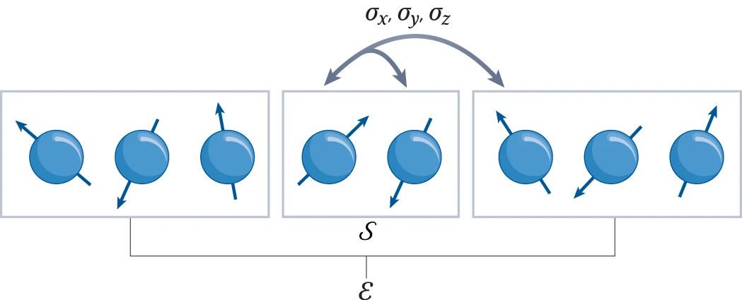
To give you a touchstone, let me present a simple example of a system with noncommuting charges. Imagine a chain of qubits, where each qubit interacts with its nearest and next-nearest neighbours, such as in the image below.

The figure is courtesy of the talented team at Nature. Two qubits form the system S of interest, and the rest form the environment E. A qubit’s three spin components, σa=x,y,z, form the local noncommuting charges. The dynamics locally transport and globally conserve the charges.

In this interaction, the qubits exchange quanta of spin angular momentum, forming what is known as a Heisenberg spin chain. This chain is characterized by three charges which are the total spin components in the x, y, and z directions, which I’ll refer to as Qx, Qy, and Qz, respectively. The Hamiltonian H conserves these charges, satisfying [H, Qa] = 0 for each a, and these three charges are non-commuting, [Qa, Qb] 0, for any pair a, b ∈ {x,y,z} where a≠b. It’s noteworthy that Hamiltonians can be constructed to transport various other kinds of noncommuting charges. I have discussed the procedure to do so in more detail here (to summarize that post: it essentially involves constructing a Koi pond).

This is the first in a series of blog posts where I will highlight key elements discussed in the perspective article. Motivated by requests from peers for a streamlined introduction to the subject, I’ve designed this series specifically for a target audience: graduate students in physics. Additionally, I’m gearing up to defending my PhD thesis on noncommuting-charge physics next semester and these blog posts will double as a fun way to prepare for that.

  1. This opening text was taken from the draft of my thesis. ↩︎

You can win Tic Tac Toe, if you know quantum physics.

Note: Oliver Zheng is a senior at University High School, Irvine CA. He has been working on AI players for quantum versions of Tic Tac Toe under the supervision of Dr. Spiros Michalakis.

Several years ago, while scrolling through YouTube, I came across a video of Paul Rudd playing something called “Quantum Chess.” I had no idea what it was, nor did I know that it would become one of the most gloriously nerdy rabbit holes I would ever fall into (see: 5D Chess with Multiverse Time Travel).

Over time, I tried to teach myself how to play these multi-layered, multi-dimensional games, but progress was slow. However, while taking a break during a piano lesson last year, I mentioned to my teacher my growing interest in unnecessarily stressful versions of chess. She told me that she happened to be friends with Dr. Xie Chen, professor of theoretical physics at Caltech who was sponsoring a Quantum Gaming project. I immediately jumped at the opportunity to connect with her, and within days was able to have my first online meeting with Dr. Chen. Soon after, I got invited to join the project. Following my introduction to the team, I started reading “Quantum Computation and Quantum Information”, which helped me understand how the theory behind the games worked. When I felt ready, Dr. Chen referred me to Dr. Spiros Michalakis at Caltech, who, funnily enough, was the creator of the quantum chess video. 

I would’ve never imagined that I am two degrees of separation from Paul Rudd, but nonetheless, I wanted to share some of the work I’ve been doing with Spiros on Quantum TiqTaqToe.

What is Quantum TiqTaqToe?

Evert van Nieuwenburg, the creator of Quantum TiqTaqToe whom I also collaborated with, goes in depth about how the game works here, but I will give a short rundown. The general idea is that there is now a split move, where you can put an ‘X’ in two different squares at once — a Schrödinger’s X, if you will. When the board has no more empty squares, the X randomly ‘collapses’ into one of the two squares with equal probability. The game ends when there are three real X’s or three real O’s in a row, just as in regular tic-tac-toe. Depending on the mode you are playing, you might also be able to entangle your X’s with your opponent’s O’s. You can get a better sense of all this by actually playing the game here.

My goal was to find out who wins when both players play optimally. For instance, in normal tic-tac-toe, it is well-known that the first X should go in the middle of the board, and if player O counters successfully, the game should end in a tie. Is the outcome of Quantum TiqTaqToe, too, predetermined to end in a tie if both players play optimally? And, if not, what is the best first move for player X? I sought to answer these questions through the power of computation.

The First Attempt

In the following section, I refer to a ‘game state’ as any unique arrangement of X’s and O’s on a board. The ‘empty game state’ simply means an empty board. ‘Traversing’ through a certain game state means that, at some point in the game, that game state occurs. So, for example, every game traverses through the empty game state, since every game starts with an empty board.

In order to solve the unsolved, one must first solve the solved. As such, my first attempt was to create an algorithm that would figure out the best move to play in regular tic-tac-toe. This first attempt was rather straightforward, and I will explain it here:

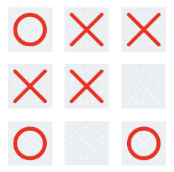
Essentially, I developed a model using what is known as “reinforcement learning” to determine the best next move given a certain game state. Here is how it works: To track which set of moves are best for player X and player O, respectively, every game state is assigned a value, initially 0. When a game ends, these values are updated to reflect who won. The more games are played, the better these values reflect the sequence of moves that X and O must make to win or tie. To train this model (machine learning parlance for the algorithm that updates the values/parameters mentioned above), I programmed the computer to play randomly chosen moves for X and O, until the game ended. If, say, player X won, then the value of every game state traversed was increased by 1 to indicate that X was favored. On the other hand, if player O won, then the value of every game state traversed was decreased by 1 to indicate that O was favored. Here is an example:

X wins!

Let’s say that this is the first iteration that the model is trained on. Then, the next time the model sees this game state,

it will recognize that X has an advantage. In the same vein, the model now also thinks that the empty game state is favorable towards X, since, in the one game that was played, when the empty game state was traversed, X won.

If we run these randomized games enough times (I ran ten million iterations), every move in every game state has most likely been made, which means that the model is able to give a meaningful evaluation for any game state. However, there is one major problem with this approach, in that the model only indicates who is favored when they make a random move, not when they make the best move. To illustrate this, let’s examine the following game state:

(O’s turn)

Here, player O has two options: they can win the game by putting their O on the bottom center square, or lose the game by putting it on the right center square. Any seasoned tic-tac-toe player would make the right move in this scenario, and win the game. However, since the model trains on random moves, it thinks that player O will win half the time and lose half the time. Thus, to the model, this game state is not favorable to either player, when in reality it is absolutely favored towards O. 

During my first meeting with Spiros and Evert, they pointed out this flaw in my model. Evert suggested that I study up on something called a minimax algorithm, which circumvents this flaw, and apply it to tic-tac-toe. This set me on the next step of my journey.

Enter Minimax

The content of this section takes inspiration from this article.

In the minimax algorithm, the two players are known as the ‘maximizer’ and the ‘minimizer’. In the case of tic-tac-toe, X would be the maximizer and O the minimizer. The maximizer’s goal is to maximize their score, while the minimizer’s goal is to minimize their score. In tic-tac-toe, the minimax algorithm is implemented so that a win by X is a score of +1, a win by O is a score of -1, and a tie is simply 0. So X, seeking to maximize their score, would want to win, which makes sense.

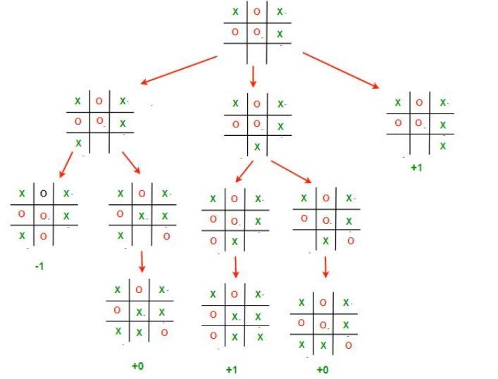
Now, if X wanted to maximize their score through some move, they would have to consider O’s move, who would try to minimize the score. But before O makes their move, they would have to consider X’s next move. This creates a sort of back-and-forth, recursive dynamic in the minimax algorithm. In order for either player to make the best move, they would have to go through all possible moves they can make, and all possible moves their opponent can make after that, and so on and so forth. Here is a relatively simple example of the minimax algorithm at work:

Let’s start from the top. X has three possible moves they can make, and evaluates each of them. 

In the leftmost branch, the result is either -1 or 0, but which is the real score? Well, we expect O to make their best move, and since they are trying to minimize the score, we expect them to choose the ‘-1’ case. So we can say that this move results in a score of -1. 

In the middle branch, the result is either 1 or 0, and, following the same reasoning as before, O chooses the move corresponding to the minimal score, resulting in a score of 0.

Finally, the last branch results in X winning, so the score is +1.

Now, X can finally choose their best move, and in the interest of maximizing the score, places their X on the bottom right square. Intuitively, this makes sense because it was the only move that wins the game for X outright.

Great, but what would a minimax algorithm look like in Quantum Tiqtaqtoe?

Enter Expecti-Minimax

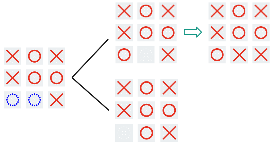
Expectiminimax contains the same core idea as minimax, but something interesting happens when the game board collapses. The algorithm can’t know for sure what the board will look like after collapse, so all it can do is calculate an expected value of the result (hence the name). Let’s look at an example:

Here, collapse occurs, and one branch (top) results in a tie, while the other (bottom) results in O winning. Since a tie is equal to 0 and an O win is equal to -1, the algorithm treats the score as

Note: the sum is divided by two because both outcomes have a ½ probability of occurring.

Solving the Game

Using the expecti-minimax algorithm, I effectively ‘solved’ the minimal and moderate versions of quantum tiqtaqtoe. However, even though the algorithm will always show the best move, the outcome from game to game might not be the same due to the inherent element of randomness. The most interesting of all my discoveries was probably the first move that the algorithm suggests for X, which I was able to make sense of both intuitively and logically. I challenge you all to find it! (Hint: it is the same for both the minimal and moderate versions.)

It turns out that when X plays optimally, they will always win the minimal version no matter what O plays. Meanwhile, in the moderate version, X will win most of the time, but not all the time. The probability distribution is as follows:

  (Another challenge: why are the denominators powers of two?)

Having satisfied my curiosity (for now), I’m looking forward to creating a new game of my own: 4 by 4 quantum tic-tac-toe. Currently, I am working on an algorithm that will give the best move, but since a 4×4 board is almost two times larger than a 3×3 board, the computational runtime of an expectiminimax algorithm would be far too large. As such, I am exploring the use of heuristics, which is sort of what the human mind uses to approach a game like tic-tac-toe. Because of this reliance on heuristics, there is no longer a guarantee that the algorithm will always make the best move, making this new adventure all the more mysterious and captivating. 

Can Thermodynamics Resolve the Measurement Problem?

At the recent Quantum Thermodynamics conference in Vienna (coming next year to the University of Maryland!), during an expert panel Q&A session, one member of the audience asked “can quantum thermodynamics address foundational problems in quantum theory?”

That stuck with me, because that’s exactly what my research is about. So naturally, I’d say the answer is yes! In fact, here in the group of Marcus Huber at the Technical University of Vienna, we think thermodynamics may have something to say about the biggest quantum foundations problem of all: the measurement problem.

It’s sort of the iconic mystery of quantum mechanics: we know that an electron can be in two places at once – in a ‘superposition’ – but when we measure it, it’s only ever seen to be in one place, picked seemingly at random from the two possibilities. We say the state has ‘collapsed’.

What’s going on here? Thanks to Bell’s legendary theorem, we know that the answer can’t just be that it was always actually in one place and we just didn’t know which option it was – it really was in two places at once until it was measured1. But also, we don’t see this effect for sufficiently large objects. So how can this ‘two-places-at-once’ thing happen at all, and why does it stop happening once an object gets big enough?

Here, we already see hints that thermodynamics is involved, because even classical thermodynamics says that big systems behave differently from small ones. And interestingly, thermodynamics also hints that the narrative so far can’t be right. Because when taken at face value, the ‘collapse’ model of measurement breaks all three laws of thermodynamics.

Imagine an electron in a superposition of two energy levels: a combination of being in its ground state and first excited state. If we measure it and it ‘collapses’ to being only in the ground state, then its energy has decreased: it went from having some average of the ground and excited energies to just having the ground energy. The first law of thermodynamics says (crudely) that energy is conserved, but the loss of energy is unaccounted for here.

Next, the second law says that entropy always increases. One form of entropy represents your lack of information about a system’s state. Before the measurement, the system was in one of two possible states, but afterwards it was in only one state. So speaking very broadly, our uncertainty about its state, and hence the entropy, is reduced. (The third law is problematic here, too.)

There’s a clear explanation here: while the system on its own decreases its entropy and doesn’t conserve energy, in order to measure something, we must couple the system to a measuring device. That device’s energy and entropy changes must account for the system’s changes.

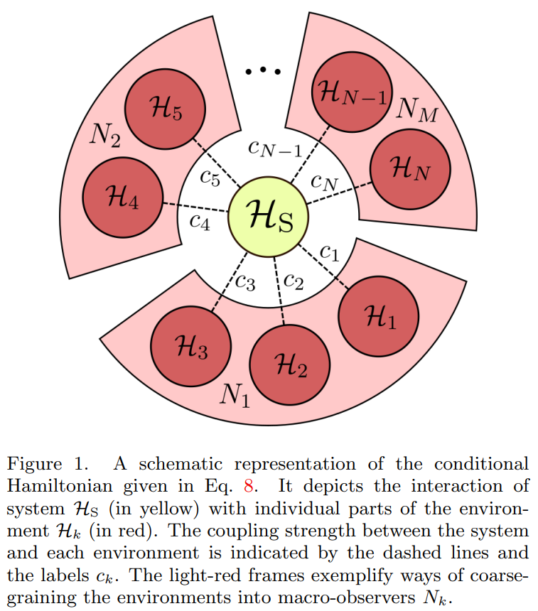
This is the spirit of our measurement model2. We explicitly include the detector as a quantum object in the record-keeping of energy and information flow. In fact, we also include the entire environment surrounding both system and device – all the lab’s stray air molecules, photons, etc. Then the idea is to describe a measurement process as propagating a record of a quantum system’s state into the surroundings without collapsing it.

A schematic representation of a system spreading information into an environment (from Schwarzhans et al., with permission)

But talking about quantum systems interacting with their environments is nothing new. The “decoherence” model from the 70s, which our work builds on, says quantum objects become less quantum when buffeted by a larger environment.

The problem, though, is that decoherence describes how information is lost into an environment, and so usually the environment’s dynamics aren’t explicitly calculated: this is called an open-system approach. By contrast, in the closed-system approach we use, you model the dynamics of the environment too, keeping track of all information. This is useful because conventional collapse dynamics seems to destroy information, but every other fundamental law of physics seems to say that information can’t be destroyed.

This all allows us to track how information flows from system to surroundings, using the “Quantum Darwinism” (QD) model of W.H. Żurek. Whereas decoherence describes how environments affect systems, QD describes how quantum systems impact their environments by spreading information into them. The QD model says that the most ‘classical’ information – the kind most consistent with classical notions of ‘being in one place’, etc. – is the sort most likely to ‘survive’ the decoherence process.

QD then further asserts that this is the information that’s most likely to be copied into the environment. If you look at some of a system’s surroundings, this is what you’d most likely see. (The ‘Darwinism’ name is because certain states are ‘selected for’ and ‘replicate’3.)

So we have a description of what we want the post-measurement state to look like: a decohered system, with its information redundantly copied into its surrounding environment. The last piece of the puzzle, then, is to ask how a measurement can create this state. Here, we finally get to the dynamics part of the thermodynamics, and introduce equilibration.

Earlier we said that even if the system’s entropy decreases, the detector’s entropy (or more broadly the environment’s) should go up to compensate. Well, equilibration maximizes entropy. In particular, equilibration describes how a system tends towards a particular ‘equilibrium’ state, because the system can always increase its entropy by getting closer to it.

It’s usually said that systems equilibrate if put in contact with an external environment (e.g. a can of beer cooling in a fridge), but we’re actually interested in a different type of equilibration called equilibration on average. There, we’re asking for the state that a system stays roughly close to, on average, over long enough times, with no outside contact. That means it never actually decoheres, it just looks like it does for certain observables. (This actually implies that nothing ever actually decoheres, since open systems are only an approximation you make when you don’t want to track all of the environment.)

Equilibration is the key to the model. In fact, we call our idea the Measurement-Equilibration Hypothesis (MEH): we’re asserting that measurement is an equilibration process. Which makes the final question: what does all this mean for the measurement problem?

In the MEH framework, when someone ‘measures’ a quantum system, they allow some measuring device, plus a chaotic surrounding environment, to interact with it. The quantum system then equilibrates ‘on average’ with the environment, and spreads information about its classical states into the surroundings. Since you are a macroscopically large human, any measurement you do will induce this sort of equilibration to happen, meaning you will only ever have access to the classical information in the environment, and never see superpositions. But no collapse is necessary, and no information is lost: rather some information is only much more difficult to access in all the environment noise, as happens all the time in the classical world.

It’s tempting to ask what ‘happens’ to the outcomes we don’t see, and how nature ‘decides’ which outcome to show to us. Those are great questions, but in our view, they’re best left to philosophers4. For the question we care about: why measurements look like a ‘collapse’, we’re just getting started with our Measurement-Equilibration Hypothesis – there’s still lots to do in our explorations of it. We think the answers we’ll uncover in doing so will form an exciting step forward in our understanding of the weird and wonderful quantum world.

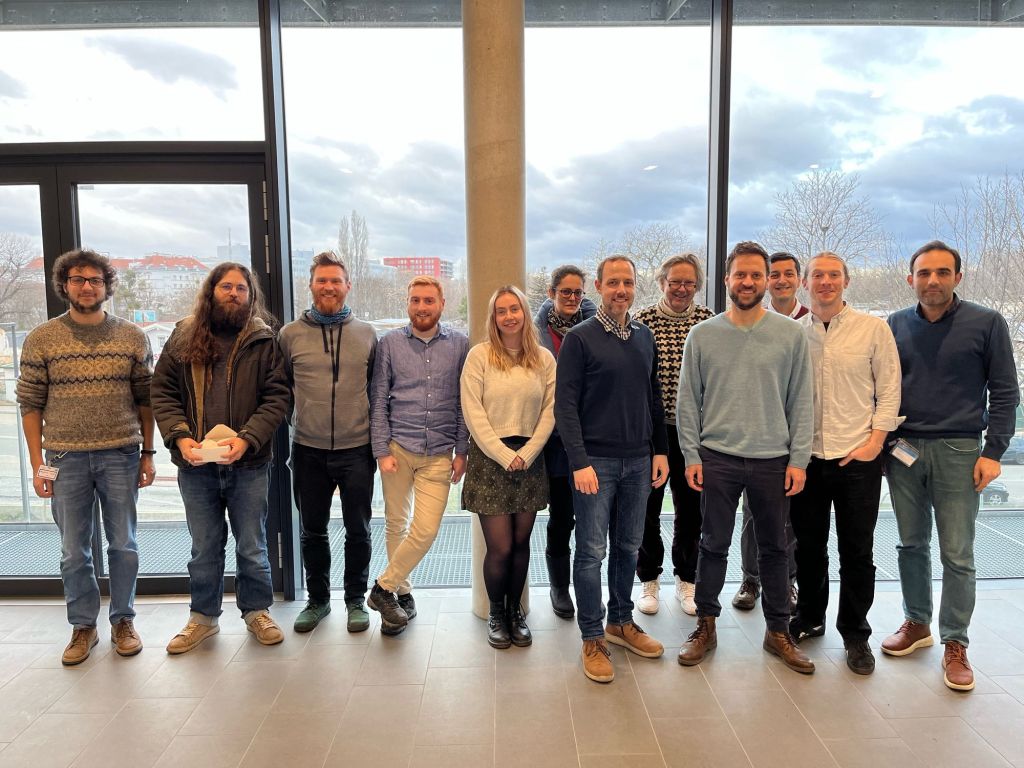
Members of the MEH team at a kick-off meeting for the project in Vienna in February 2023. Left to right: Alessandro Candeloro, Marcus Huber, Emanuel Schwarzhans, Tom Rivlin, Sophie Engineer, Veronika Baumann, Nicolai Friis, Felix C. Binder, Mehul Malik, Maximilian P.E. Lock, Pharnam Bakhshinezhad

Acknowledgements: Big thanks to the rest of the MEH team for all the help and support, in particular Dr. Emanuel Schwarzhans and Dr. Lock for reading over this piece!)

Here are a few choice references (by no means meant to be comprehensive!)

Quantum Thermodynamics (QTD) Conference 2023: https://qtd2023.conf.tuwien.ac.at/
QTD 2024: https://qtd-hub.umd.edu/event/qtd-conference-2024/
Bell’s Theorem: https://plato.stanford.edu/entries/bell-theorem/
The first MEH paper: https://arxiv.org/abs/2302.11253
A review of decoherence: https://journals.aps.org/rmp/abstract/10.1103/RevModPhys.75.715
Quantum Darwinism: https://www.nature.com/articles/nphys1202
Measurements violate the 3rd law: https://quantum-journal.org/papers/q-2020-01-13-222/
More on the 3rd and QM: https://journals.aps.org/prxquantum/abstract/10.1103/PRXQuantum.4.010332
Equilibration on average: https://iopscience.iop.org/article/10.1088/0034-4885/79/5/056001/meta
Objectivity: https://journals.aps.org/pra/abstract/10.1103/PhysRevA.91.032122

  1. There is a perfectly valid alternative with other weird implications: that it was always just in one place, but the world is intrinsically non-local. Most physicists prefer to save locality over realism, though. ↩︎
  2. First proposed in this paper by Schwarzhans, Binder, Huber, and Lock: https://arxiv.org/abs/2302.11253 ↩︎
  3. In my opinion… it’s a brilliant theory with a terrible name! Sure, there’s something akin to ‘selection pressure’ and ‘reproduction’, but there aren’t really any notions of mutation, adaptation, fitness, generations… Alas, the name has stuck. ↩︎
  4. I actually love thinking about this question, and the interpretations of quantum mechanics more broadly, but it’s fairly orthogonal to the day-to-day research on this model. ↩︎

Caltech’s Ginsburg Center

Editor’s note: On 10 August 2023, Caltech celebrated the groundbreaking for the Dr. Allen and Charlotte Ginsburg Center for Quantum Precision Measurement, which will open in 2025. At a lunch following the ceremony, John Preskill made these remarks.

Rendering of the facade of the Ginsburg Center

Hello everyone. I’m John Preskill, a professor of theoretical physics at Caltech, and I’m honored to have this opportunity to make some brief remarks on this exciting day.

In 2025, the Dr. Allen and Charlotte Ginsburg Center for Quantum Precision Measurement will open on the Caltech campus. That will certainly be a cause for celebration. Quite fittingly, in that same year, we’ll have something else to celebrate — the 100th anniversary of the formulation of quantum mechanics in 1925. In 1900, it had become clear that the physics of the 19th century had serious shortcomings that needed to be addressed, and for 25 years a great struggle unfolded to establish a firm foundation for the science of atoms, electrons, and light; the momentous achievements of 1925 brought that quest to a satisfying conclusion. No comparably revolutionary advance in fundamental science has occurred since then.

For 98 years now we’ve built on those achievements of 1925 to arrive at a comprehensive understanding of much of the physical world, from molecules to materials to atomic nuclei and exotic elementary particles, and much else besides. But a new revolution is in the offing. And the Ginsburg Center will arise at just the right time and at just the right place to drive that revolution forward.

Up until now, most of what we’ve learned about the quantum world has resulted from considering the behavior of individual particles. A single electron propagating as a wave through a crystal, unfazed by barriers that seem to stand in its way. Or a single photon, bouncing hundreds of times between mirrors positioned kilometers apart, dutifully tracking the response of those mirrors to gravitational waves from black holes that collided in a galaxy billions of light years away. Understanding that single-particle physics has enabled us to explore nature in unprecedented ways, and to build information technologies that have profoundly transformed our lives.

At the groundbreaking: Physics, Math and Astronomy Chair Fiona Harrison, California Assemblymember Chris Holden, President Tom Rosenbaum, Charlotte Ginsburg, Dr. Allen Ginsburg, Pasadena Mayor Victor Gordo, Provost Dave Tirrell.

What’s happening now is that we’re getting increasingly adept at instructing particles to move in coordinated ways that can’t be accurately described in terms of the behavior of one particle at a time. The particles, as we like to say, can become entangled. Many particles, like electrons or photons or atoms, when highly entangled, exhibit an extraordinary complexity that we can’t capture with the most powerful of today’s supercomputers, or with our current theories of how Nature works. That opens extraordinary opportunities for new discoveries and new applications.

We’re very proud of the role Caltech has played in setting the stage for the next quantum revolution. Richard Feynman envisioning quantum computers that far surpass the computers we have today. Kip Thorne proposing ways to use entangled photons to perform extraordinarily precise measurements. Jeff Kimble envisioning and executing ingenious methods for entangling atoms and photons. Jim Eisenstein creating and studying extraordinary phenomena in a soup of entangled electrons. And much more besides. But far greater things are yet to come.

How can we learn to understand and exploit the behavior of many entangled particles that work together? For that, we’ll need many scientists and engineers who work together. I joined the Caltech faculty in August 1983, almost exactly 40 years ago. These have been 40 good years, but I’m having more fun now than ever before. My training was in elementary particle physics. But as our ability to manipulate the quantum world advances, I find that I have more and more in common with my colleagues from different specialties. To fully realize my own potential as a researcher and a teacher, I need to stay in touch with atomic physics, condensed matter physics, materials science, chemistry, gravitational wave physics, computer science, electrical engineering, and much else. Even more important, that kind of interdisciplinary community is vital for broadening the vision of the students and postdocs in our research groups.

Nurturing that community — that’s what the Ginsburg Center is all about. That’s what will happen there every day. That sense of a shared mission, enhanced by colocation, will enable the Ginsburg Center to lead the way as quantum science and technology becomes increasingly central to Caltech’s research agenda in the years ahead, and increasingly important for science and engineering around the globe. And I just can’t wait for 2025.

Caltech is very fortunate to have generous and visionary donors like the Ginsburgs and the Sherman Fairchild Foundation to help us realize our quantum dreams.

Dr. Allen and Charlotte Ginsburg

Identical twins and quantum entanglement

“If I had a nickel for every unsolicited and very personal health question I’ve gotten at parties, I’d have paid off my medical school loans by now,” my doctor friend complained. As a physicist, I can somewhat relate. I occasionally find myself nodding along politely to people’s eccentric theories about the universe. A gentleman once explained to me how twin telepathy (the phenomenon where, for example, one twin feels the other’s pain despite being in separate countries) comes from twins’ brains being entangled in the womb. Entanglement is a nonclassical correlation that can exist between spatially separated systems. If two objects are entangled, it’s possible to know everything about both of them together but nothing about either one. Entangling two particles (let alone full brains) over tens of kilometres (let alone full countries) is incredibly challenging. “Using twins to study entanglement, that’ll be the day,” I thought. Well, my last paper did something like that. 

In theory, a twin study consists of two people that are as identical as possible in every way except for one. What that allows you to do is isolate the effect of that one thing on something else. Aleksander Lasek (postdoc at QuICS), David Huse (professor of physics at Princeton), Nicole Yunger Halpern (NIST physicist and Quantum Frontiers blogger), and I were interested in isolating the effects of quantities’ noncommutation (explained below) on entanglement. To do so, we first built a pair of twins and then compared them

Consider a well-insulated thermos filled with soup. The heat and the number of “soup particles” inside the thermos are conserved. So the energy and the number of “soup particles” are conserved quantities. In classical physics, conserved quantities commute. This means that we can simultaneously measure the amount of each conserved quantity in our system, like the energy and number of soup particles. However, in quantum mechanics, this needn’t be true. Measuring one property of a quantum system can change another measurement’s outcome.

Conserved quantities’ noncommutation in thermodynamics has led to some interesting results. For example, it’s been shown that conserved quantities’ noncommutation can decrease the rate of entropy production. For the purposes of this post, entropy production is something that limits engine efficiency—how well engines can convert fuel to useful work. For example, if your car engine had zero entropy production (which is impossible), it would convert 100% of the energy in your car’s fuel into work that moved your car along the road. Current car engines can convert about 30% of this energy, so it’s no wonder that people are excited about the prospective application of decreasing entropy production. Other results (like this one and that one) have connected noncommutation to potentially hindering thermalization—the phenomenon where systems interact until they have similar properties, like when a cup of coffee cools. Thermalization limits memory storage and battery lifetimes. Thus, learning how to resist thermalization could also potentially lead to better technologies, such as longer-lasting batteries. 

One can measure the amount of entanglement within a system, and as quantum particles thermalize, they entangle. Given the above results about thermalization, we might expect that noncommutation would decrease entanglement. Testing this expectation is where the twins come in.

Say we built a pair of twins that were identical in every way except for one. Nancy, the noncommuting twin, has some features that don’t commute, say, her hair colour and height. This means that if we measure her height, we’ll have no idea what her hair colour is. For Connor, the commuting twin, his hair colour and height commute, so we can determine them both simultaneously. Which twin has more entanglement? It turns out it’s Nancy.

Disclaimer: This paragraph is written for an expert audience. Our actual models consist of 1D chains of pairs of qubits. Each model has three conserved quantities (“charges”), which are sums over local charges on the sites. In the noncommuting model, the three local charges are tensor products of Pauli matrices with the identity (XI, YI, ZI). In the commuting model, the three local charges are tensor products of the Pauli matrices with themselves (XX, YY, ZZ). The paper explains in what sense these models are similar. We compared these models numerically and analytically in different settings suggested by conventional and quantum thermodynamics. In every comparison, the noncommuting model had more entanglement on average.

Our result thus suggests that noncommutation increases entanglement. So does charges’ noncommutation promote or hinder thermalization? Frankly, I’m not sure. But I’d bet the answer won’t be in the next eccentric theory I hear at a party.

Building a Koi pond with Lie algebras

When I was growing up, one of my favourite places was the shabby all-you-can-eat buffet near our house. We’d walk in, my mom would approach the hostess to explain that, despite my being abnormally large for my age, I qualified for kids-eat-free, and I would peel away to stare at the Koi pond. The display of different fish rolling over one another was bewitching. Ten-year-old me would have been giddy to build my own Koi pond, and now I finally have. However, I built one using Lie algebras.

The different fish swimming in the Koi pond are, in many ways, like charges being exchanged between subsystems. A “charge” is any globally conserved quantity. Examples of charges include energy, particles, electric charge, or angular momentum. Consider a system consisting of a cup of coffee in your office. The coffee will dynamically exchange charges with your office in the form of heat energy. Still, the total energy of the coffee and office is conserved (assuming your office walls are really well insulated). In this example, we had one type of charge (heat energy) and two subsystems (coffee and office). Consider now a closed system consisting of many subsystems and many different types of charges. The closed system is like the finite Koi pond with different charges like the different fish species. The charges can move around locally, but the total number of charges is globally fixed, like how the fish swim around but can’t escape the pond. Also, the presence of one type of charge can alter another’s movement, just as a big fish might block a little one’s path. 

Unfortunately, the Koi pond analogy reaches its limit when we move to quantum charges. Classically, charges commute. This means that we can simultaneously determine the amount of each charge in our system at each given moment. In quantum mechanics, this isn’t necessarily true. In other words, classically, I can count the number of glossy fish and matt fish. But, in quantum mechanics, I can’t.

So why does this matter? Subsystems exchanging charges are prevalent in thermodynamics. Quantum thermodynamics extends thermodynamics to include small systems and quantum effects. Noncommutation underlies many important quantum phenomena. Hence, studying the exchange of noncommuting charges is pivotal in understanding quantum thermodynamics. Consequently, noncommuting charges have emerged as a rapidly growing subfield of quantum thermodynamics. Many interesting results have been discovered from no longer assuming that charges commute (such as these). Until recently, most of these discoveries have been theoretical. Bridging these discoveries to experimental reality requires Hamiltonians (functions that tell you how your system evolves in time) that move charges locally but conserve them globally. Last year it was unknown whether these Hamiltonians exist, what they look like generally, how to build them, and for what charges you could find them.

Nicole Yunger Halpern (NIST physicist, my co-advisor, and Quantum Frontiers blogger) and I developed a prescription for building Koi ponds for noncommuting charges. Our prescription allows you to systematically build Hamiltonians that overtly move noncommuting charges between subsystems while conserving the charges globally. These Hamiltonians are built using Lie algebras, abstract mathematical tools that can describe many physical quantities (including everything in the standard model of particle physics and space-time metric). Our results were recently published in npj QI. We hope that our prescription will bolster the efforts to bridge the results of noncommuting charges to experimental reality.

In the end, a little group theory was all I needed for my Koi pond. Maybe I’ll build a treehouse next with calculus or a remote control car with combinatorics.