Machine learning the arXiv

Over the last year or so, the machine learning wave has really been sweeping through the field of condensed matter physics. Machine learning techniques have been applied to condensed matter physics before, but very sparsely and with little recognition. These days, I guess (partially) due to the general machine learning and AI hype, the amount of such studies skyrocketed (I admit to contributing to that..). I’ve been keeping track of this using the arXiv and Twitter (@Evert_v_N), but you should know about this website for getting an overview of the physics & machine learning papers: https://physicsml.github.io/pages/papers.html.

This effort of applying machine learning to physics is a serious attempt at trying to understand how such tools could be useful in a variety of ways. It isn’t very hard to get a neural network to learn ‘something’ from physics data, but it is really hard to find out what – and especially how – the network does that. That’s why toy cases such as the Ising model or the Kosterlitz-Thouless transition have been so important!

When you’re keeping track of machine learning and AI developments, you soon realize that there are examples out there of amazing feats. Being able to generate photo-realistic pictures given just a sentence. e.g. “a brown bird with golden speckles and red wings is sitting on a yellow flower with pointy petals”, is (I think..) pretty cool. I can’t help but wonder if we’ll get to a point where we can ask it to generate “the groundstate of the Heisenberg model on a Kagome lattice of 100×100”…

Another feat I want to mention, and the main motivation for this post, is that of being able to encode words as vectors. That doesn’t immediately seem like a big achievement, but it is once you want to have ‘similar’ words have ‘similar’ vectors. That is, you intuitively understand that Queen and King are very similar, but differ basically only in gender. Can we teach that to a computer (read: neural network) by just having it read some text? Turns out we can. The general encoding of words to vectors is aptly named ‘Word2Vec’, and some of the top algorithms that do that were introduced here (https://arxiv.org/abs/1301.3781) and here (https://arxiv.org/abs/1310.4546). The neat thing is that we can actually do arithmetics with these words encoded as vectors, so that the network learns (with no other input than text!):

  • King – Man + Woman = Queen
  • Paris – France + Italy = Rome

In that spirit, I wondered if we can achieve the same thing with physics jargon. Everyone knows, namely, that “electrons + two dimensions + magnetic field = Landau levels”. But is that clear from condensed matter titles?

Try it yourself

If you decide at this point that the rest of the blog is too long, at least have a look here: everthemore.pythonanywhere.com or skip to the last section. That website demonstrates the main point of this post. If that sparks your curiosity, read on!

This post is mainly for entertainment, and so a small disclaimer is in order: in all of the results below, I am sure things can be improved upon. Consider this a ‘proof of principle’. However, I would be thrilled to see what kind of trained models you can come up with yourself! So for that purpose, all of the code (plus some bonus content!) can be found on this github repository: https://github.com/everthemore/physics2vec.

Harvesting the arXiv

The perfect dataset for our endeavor can be found in the form of the arXiv. I’ve written a small script (see github repository) that harvests the titles of a given section from the arXiv. It also has options for getting the abstracts, but I’ll leave that for a separate investigation. Note that in principle we could also get the source-files of all of these papers, but doing that in bulk requires a payment; and getting them one by one will 1) take forever and 2) probably get us banned.

Collecting all this data of the physics:cond-mat subsection took right about 1.5 hours and resulted in 240737 titles and abstracts (I last ran this script on November 20th, 2017). I’ve filtered them by year and month, and you can see the result in Fig.1 below. Seems like we have some catching up to do in 2017 still (although as the inset shows, we have nothing to fear. November is almost over, but we still have the ‘getting things done before x-mas’ rush coming up!).

numpapers

Figure 1: The number of papers in the cond-mat arXiv section over the years. We’re behind, but the year isn’t over yet! (Data up to Nov 20th 2017)

Analyzing n-grams

After tidying up the titles (removing LaTeX, converting everything to lowercase, etc.), the next thing to do is to train a language model on finding n-grams. N-grams are basically fixed n-word expressions such as ‘cooper pair’ (bigram) or ‘metal insulator transition’ (trigram). This makes it easier to train a Word2Vec encoding, since these phrases are fixed and can be considered a single word. The python module we’ll use for Word2Vec is gensim (https://radimrehurek.com/gensim/), and it conveniently has phrase-detection built-in. The language model it builds reports back to us the n-grams it finds, and assigns them a score indicating how certain it is about them. Notice that this is not the same as how frequently it appears in the dataset. Hence an n-gram can appear fewer times than another, but have a higher certainty because it always appears in the same combination. For example, ‘de-haas-van-alphen’ appears less than, but is more certain than, ‘cooper-pair’, because ‘pair’ does not always come paired (pun intended) with ‘cooper’. I’ve analyzed up to 4-grams in the analysis below.

I can tell you’re curious by now to find out what some of the most certain n-grams in cond-mat are (again, these are not necessarily the most frequent), so here are some interesting findings:

  • The most certain n-grams are all surname combo’s, Affleck-Kennedy-Lieb-Tasaki being the number 1. Kugel-Khomskii is the most certain 2-name combo and Einstein-Podolksi-Rosen the most certain 3-name combo.
  • The first certain non-name n-gram is a ‘quartz tuning fork’, followed by a ‘superconducting coplanar waveguide resonator’. Who knew.
  • The bigram ‘phys. rev.’ and trigram ‘phys. rev. lett.’ are relatively high up in the confidence lists. These seem to come from the “Comment on […]”-titles on the arXiv.
  • I learned that there is such a thing as a Lefschetz thimble. I also learned that those things are called thimbles in English (we (in Holland) call them ‘finger-hats’!).

In terms of frequency however, which is probably more of interest to us, the most dominant n-grams are Two-dimensional, Quantum dot, Phase transition, Magnetic field, One dimensional and Bose-Einstein (in descending order). It seems 2D is still more popular than 1D, and all in all the top n-grams do a good job at ‘defining’ condensed matter physics. I’ll refer you to the github repository code if you want to see a full list! You’ll find there a piece of code that produces wordclouds from the dominant words and n-grams too, such as this one:

caltechwordcloud.png

For fun though, before we finally get to the Word2Vec encoding, I’ve also kept track of all of these as a function of year, so that we can now turn to finding out which bigrams have been gaining the most popularity. The table below shows the top 5 n-grams for the period 2010 – 2016 (not including 2017) and for the period 2015 – Nov 20th 2017.

2010-2016

2015 – November 20th 2017

Spin liquids  Topological phases & transitions
 Weyl semimetals  Spin chains
 Topological phases & transitions  Machine learning
 Surface states  Transition metal dichalcogenides
 Transition metal dichalcogenides  Thermal transport
 Many-body localization  Open quantum systems

Actually, the real number 5 in the left column was ‘Topological insulators’, but given number 3 I skipped it. Also, this top 5 includes a number 6 (!), which I just could not leave off given that everyone seems to have been working on MBL. If we really want to be early adopters though, taking only the last 1.8 years (2015 – now, Nov 20th 2017)  in the right column of the table shows some interesting newcomers. Surprisingly, many-body localization is not even in the top 20 anymore. Suffice it to say, if you have been working on anything topology-related, you have nothing to worry about. Machine learning is indeed gaining lots of attention, but we’ve yet to see if it doesn’t go the MBL-route (I certainly don’t hope so!). Quantum computing does not seem to be on the cond-mat radar, but I’m certain we would find that high up in the quant-ph arXiv section.

CondMat2Vec

Alright, finally time to use some actual neural networks for machine learning. As I started this post, what we’re about to do is try to train a network to encode/decode words into vectors, while simultaneously making sure that similar words (by meaning!) have similar vectors. Now that we have the n-grams, we want the Word2Vec algorithm to treat these as words by themselves (they are, after all, fixed combinations).

In the Word2Vec algorithm, we get to decide the length of the vectors that encode words ourselves. Larger vectors means more freedom in encoding words, but also makes it harder to learn similarity. In addition, we get to choose a window-size, indicating how many words the algorithm will look ahead to analyze relations between words. Both of these parameters are free for you to play with if you have a look at the source code repository. For the website everthemore.pythonanywhere.com, I’ve uploaded a size 100 with window-size 10 model, which I found to produce sensible results. Sensible here means “based on my expectations”, such as the previous example of “2D + electrons + magnetic field = Landau levels”. Let’s ask our network some questions.

First, as a simple check, let’s see what our encoding thinks some jargon is similar to:

  • Superconductor ~ Superconducting, Cuprate superconductor, Superconductivity, Layered superconductor, Unconventional superconductor, Superconducting gap, Cuprate, Weyl semimetal, …
  • Majorana ~ Majorana fermion, Majorana mode, Non-abelian, Zero-energy, braiding, topologically protected, …

It seems we could start to cluster words based on this. But the real test comes now, in the form of arithmetics. According to our network (I am listing the top two choices in some cases; the encoder outputs a list of similar vectors, ordered by similarity):

  • Majorana + Braiding = Non-Abelian
  • Electron + Hole = Exciton, Carrier
  • Spin + Magnetic field = Magnetization, Antiferromagnetic
  • Particle + Charge = Electron, Charged particle

And, sure enough:

  • 2D + electrons + magnetic field = Landau level, Magnetoresistance oscillation

The above is just a small sample of the things I’ve tried. See the link in the try it yourself section above if you want to have a go. Not all of the examples work nicely. For example, neither lattice + wave nor lattice + excitation nor lattice + force seem to result in anything related to the word ‘phonon’. I would guess that increasing the window size will help remedy this problem. Even better probably would be to include abstracts!

Outlook

I could play with this for hours, and I’m sure that by including the abstracts and tweaking the vector size (plus some more parameters I haven’t even mentioned) one could optimize this more. Once we have an optimized model, we could start to cluster the vectors to define research fields, visualizing the relations between n-grams (both suggestions thanks to Thomas Vidick and John Preskill!), and many other things. This post has become rather long already however, and I will leave further investigation to a possible future post. I’d be very happy to incorporate anything cool you find yourselves though, so please let me know!

Gently yoking yin to yang

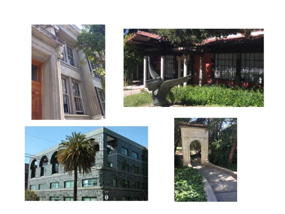
The architecture at the University of California, Berkeley mystified me. California Hall evokes a Spanish mission. The main library consists of white stone pillared by ionic columns. A sea-green building scintillates in the sunlight like a scarab. The buildings straddle the map of styles.

Architecture.001

So do Berkeley’s quantum scientists, information-theory users, and statistical mechanics.

The chemists rove from abstract quantum information (QI) theory to experiments. Physicists experiment with superconducting qubits, trapped ions, and numerical simulations. Computer scientists invent algorithms for quantum computers to perform.

Few activities light me up more than bouncing from quantum group to info-theory group to stat-mech group, hunting commonalities. I was honored to bounce from group to group at Berkeley this September.

What a trampoline Berkeley has.

The groups fan out across campus and science, but I found compatibility. Including a collaboration that illuminated quantum incompatibility.

Quantum incompatibility originated in studies by Werner Heisenberg. He and colleagues cofounded quantum mechanics during the early 20th century. Measuring one property of a quantum system, Heisenberg intuited, can affect another property.

The most famous example involves position and momentum. Say that I hand you an electron. The electron occupies some quantum state represented by | \Psi \rangle. Suppose that you measure the electron’s position. The measurement outputs one of many possible values x (unless | \Psi \rangle has an unusual form, the form a Dirac delta function).

But we can’t say that the electron occupies any particular point x = x_0 in space. Measurement devices have limited precision. You can measure the position only to within some error \varepsilon: x = x_0 \pm \varepsilon.

Suppose that, immediately afterward, you measure the electron’s momentum. This measurement, too, outputs one of many possible values. What probability q(p) dp does the measurement have of outputting some value p? We can calculate q(p) dp, knowing the mathematical form of | \Psi \rangle and knowing the values of x_0 and \varepsilon.

q(p) is a probability density, which you can think of as a set of probabilities. The density can vary with p. Suppose that q(p) varies little: The probabilities spread evenly across the possible p values. You have no idea which value your momentum measurement will output. Suppose, instead, that q(p) peaks sharply at some value p = p_0. You can likely predict the momentum measurement’s outcome.

The certainty about the momentum measurement trades off with the precision \varepsilon of the position measurement. The smaller the \varepsilon (the more precisely you measured the position), the greater the momentum’s unpredictability. We call position and momentum complementary, or incompatible.

You can’t measure incompatible properties, with high precision, simultaneously. Imagine trying to do so. Upon measuring the momentum, you ascribe a tiny range of momentum values p to the electron. If you measured the momentum again, an instant later, you could likely predict that measurement’s outcome: The second measurement’s q(p) would peak sharply (encode high predictability). But, in the first instant, you measure also the position. Hence, by the discussion above, q(p) would spread out widely. But we just concluded that q(p) would peak sharply. This contradiction illustrates that you can’t measure position and momentum, precisely, at the same time.

But you can simultaneously measure incompatible properties weakly. A weak measurement has an enormous \varepsilon. A weak position measurement barely spreads out q(p). If you want more details, ask a Quantum Frontiers regular; I’ve been harping on weak measurements for months.

Blame Berkeley for my harping this month. Irfan Siddiqi’s and Birgitta Whaley’s groups collaborated on weak measurements of incompatible observables. They tracked how the measured quantum state | \Psi (t) \rangle evolved in time (represented by t).

Irfan’s group manipulates superconducting qubits.1 The qubits sit in the physics building, a white-stone specimen stamped with an egg-and-dart motif. Across the street sit chemists, including members of Birgitta’s group. The experimental physicists and theoretical chemists teamed up to study a quantum lack of teaming up.

Phys. & chem. bldgs

The experiment involved one superconducting qubit. The qubit has properties analogous to position and momentum: A ball, called the Bloch ball, represents the set of states that the qubit can occupy. Imagine an arrow pointing from the sphere’s center to any point in the ball. This Bloch vector represents the qubit’s state. Consider an arrow that points upward from the center to the surface. This arrow represents the qubit state | 0 \rangle. | 0 \rangle is the quantum analog of the possible value 0 of a bit, or unit of information. The analogous downward-pointing arrow represents the qubit state | 1 \rangle, analogous to 1.

Infinitely many axes intersect the sphere. Different axes represent different observables that Irfan’s group can measure. Nonparallel axes represent incompatible observables. For example, the x-axis represents an observable \sigma_x analogous to position. The y-axis represents an observable \sigma_y analogous to momentum.

Tug-of-war

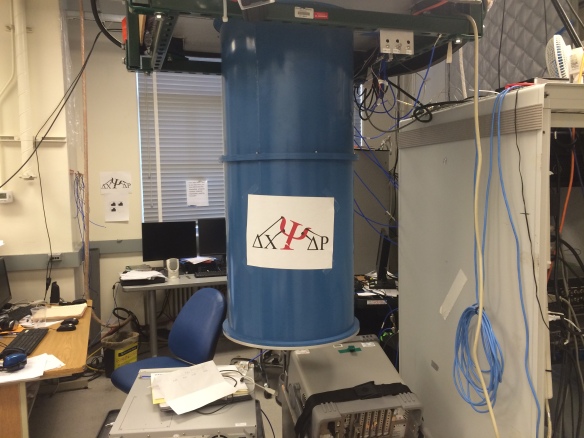
Siddiqi lab, decorated with the trademark for the paper’s tug-of-war between incompatible observables. Photo credit: Leigh Martin, one of the paper’s leading authors.

Irfan’s group stuck their superconducting qubit in a cavity, or box. The cavity contained light that interacted with the qubit. The interactions transferred information from the qubit to the light: The light measured the qubit’s state. The experimentalists controlled the interactions, controlling the axes “along which” the light was measured. The experimentalists weakly measured along two axes simultaneously.

Suppose that the axes coincided—say, at the x-axis \hat{x}. The qubit would collapse to the state | \Psi \rangle = \frac{1}{ \sqrt{2} } ( | 0 \rangle + | 1 \rangle ), represented by the arrow that points along \hat{x} to the sphere’s surface, or to the state | \Psi \rangle = \frac{1}{ \sqrt{2} } ( | 0 \rangle - | 1 \rangle ), represented by the opposite arrow.

0 deg

(Projection of) the Bloch Ball after the measurement. The system can access the colored points. The lighter a point, the greater the late-time state’s weight on the point.

Let \hat{x}' denote an axis near \hat{x}—say, 18° away. Suppose that the group weakly measured along \hat{x} and \hat{x}'. The state would partially collapse. The system would access points in the region straddled by \hat{x} and \hat{x}', as well as points straddled by - \hat{x} and - \hat{x}'.

18 deg

Finally, suppose that the group weakly measured along \hat{x} and \hat{y}. These axes stand in for position and momentum. The state would, loosely speaking, swirl around the Bloch ball.

90 deg

The Berkeley experiment illuminates foundations of quantum theory. Incompatible observables, physics students learn, can’t be measured simultaneously. This experiment blasts our expectations, using weak measurements. But the experiment doesn’t just destroy. It rebuilds the blast zone, by showing how | \Psi (t) \rangle evolves.

“Position” and “momentum” can hang together. So can experimentalists and theorists, physicists and chemists. So, somehow, can the California mission and the ionic columns. Maybe I’ll understand the scarab building when we understand quantum theory.2

With thanks to Birgitta’s group, Irfan’s group, and the rest of Berkeley’s quantum/stat-mech/info-theory community for its hospitality. The Bloch-sphere figures come from http://www.nature.com/articles/nature19762.

1The qubit is the quantum analog of a bit. The bit is the basic unit of information. A bit can be in one of two possible states, which we can label as 0 and 1. Qubits can manifest in many physical systems, including superconducting circuits. Such circuits are tiny quantum circuits through which current can flow, without resistance, forever.

2Soda Hall dazzled but startled me.

Majorana update

If you are, by any chance, following progress in the field of Majorana bound states, then you are for sure super excited about ample Majorana results arriving this Fall. On the other hand, if you just heard about these elusive states recently, it is time for an update. For physicists working in the field, this Fall was perhaps the most exciting time since the first experimental reports from 2012. In the last few weeks there was not only one, but at least three interesting manuscripts reporting new insightful data which may finally provide a definitive experimental verification of the existence of these states in condensed matter systems.

But before I dive into these new results, let me give a brief history on the topic of  Majorana states and their experimental observation. The story starts with the young talented physicist Ettore Majorana, who hypothesized back in 1937 the existence of fermionic particles which were their own antiparticles. These hypothetical particles, now called Majorana fermions, were proposed in the context of elementary particle physics, but never observed. Some 60 years later, in the early 2000s, theoretical work emerged showing that Majorana fermionic states can exist as the quasiparticle excitations in certain low-dimensional superconducting systems (not a real particle as originally proposed, but otherwise having the exact same properties). Since then theorists have proposed half a dozen possible ways to realize Majorana modes using readily available materials such as superconductors, semiconductors, magnets, as well as topological insulators (for curious readers, I recommend manuscripts [1, 2, 3] for an overview of the different proposed methods to realize Majorana states in the lab).

The most fascinating thing about Majorana states is that they belong to the class of anyons, which means that they behave neither as bosons nor as fermions upon exchange. For example, if you have two identical fermionic (or bosonic) states and you exchange their positions, the quantum mechanical function describing the two states will acquire a phase factor of -1 (or +1). Anyons, on the other hand, can have an arbitrary phase factor eiφ upon exchange. For this reason, they are considered to be a starting point for topological quantum computation. If you want to learn more about anyons, check out the video below featuring IQIM’s Gil Refael and Jason Alicea.


Back in 2012, a group in Delft (led by Prof. Leo Kouwenhoven) announced the observation of zero-energy states in a nanoscale device consisting of a semiconductor nanowire coupled to a superconductor. These states behaved very similarly to the Majoranas that were previously predicted to occur in this system. The key word here is ‘similar’, since the behavior of these modes was not fully consistent with the theoretical predictions. Namely, the electrical conductance carried through the observed zero energy states was only about ~5% of the expected perfect transmission value for Majoranas. This part of the data was very puzzling, and immediately cast some doubts throughout the community. The physicists were quickly divided into what I will call enthusiasts (believers that these initial results indeed originated from Majorana states) and skeptics (who were pointing out that effects, other than Majoranas, can result in similarly looking zero energy peaks). And thus a great debate started.

In the coming years, experimentalists tried to observe zero energy features in improved devices, track how these features evolve with external parameters, such as gate voltages, length of the wires, etc., or focus on completely different platforms for hosting Majorana states, such as magnetic flux vortices in topological superconductors and magnetic atomic chains placed on a superconducting surface.  However, these results were not enough to convince skeptics that the observed states indeed originated from the Majoranas and not some other yet-to-be-discovered phenomenon. And so, the debate continued. With each generation of the experiments some of the alternative proposed scenarios were ruled out, but the final verification was still missing.

Fast forward to the events of this Fall and the exciting recent results. The manuscript I would like to invite you to read was just posted on ArXiv a couple of weeks ago. The main result is the observation of the perfectly quantized 2e2/h conductance at zero energy, the long sought signature of the Majorana states. This quantization implies that in this latest generation of semiconducting-superconducting devices zero-energy states exhibit perfect electron-hole symmetry and thus allow for perfect Andreev reflection. These remarkable results may finally end the debate and convince most of the skeptics out there.

Fig_blog

Figure 1. (a,b) Comparison between devices and measurements from 2012 and 2017. (a) In 2012 a device made by combining a superconductor (Niobium Titanium Nitride alloy) and Indium Antimonide nanowire resulted in the first signature of zero energy states but the conductance peak was only about 0.1 x e2/h. Adapted from Mourik et al. Science 2012. (b) Similar device from 2017 made by carefully depositing superconducting Aluminum on Indium Arsenide. The fully developed 2e2/h conductance peak was observed. Adapted from Zhang et. al. ArXiv 2017. (c) Schematics of the Andreev reflection through the Normal (N)/Superconductor (S) interface. (d,e) Alternative view of the Andreev reflection process as a tunneling through a double barrier without and with Majorana modes (shown in yellow).

To fully appreciate these results, it is useful to quickly review the physics of Andreev reflection (Fig. 1c-e) that occurs at the interface between a normal region with a superconductor [4]. As the electron (blue) in the normal region enters a superconductor and pulls an additional electron with it to form a Copper pair, an extra hole (red) is left behind (Fig. 1(c)). You can also think about this process as the transmission through two leads, one connecting the superconductor to the electrons and the other to the holes (Fig. 1d). This allows us to view this problem as a transmission through the double barrier that is generally low. In the presence of a Majorana state, however, there is a resonant level at zero energy which is coupled with the same amplitude with both electrons and holes. This in turn results in the resonant Andreev reflection with a perfect quantization of 2e2/h (Fig. 1e). Note that, even in the configuration without Majorana modes, perfect quantization is possible but highly unlikely as it requires very careful tuning of the barrier potential (the authors did show that their quantization is robust against tuning the voltages on the gates, ruling out this possibility).

Going back to the experiments, you may wonder what made this breakthrough possible? It seems to be the combination of various factors, including using epitaxially grown  superconductors and more sophisticated fabrication methods. As often happens in experimental physics, this milestone did not come from one ingenious idea, but rather from numerous technical improvements obtained by several generations of hard-working grad students and postdocs.

If you are up for more Majorana reading, you can find two more recent eye-catching manuscripts here and here. Note that the list of interesting recent Majorana papers is a mere selection by the author and not complete by any means. A few months ago, my IQIM colleagues wrote a nice blog entry about topological qubits arriving in 2018. Although this may sound overly optimistic, the recent results suggest that the field is definitely taking off. While there are certainly many challenges to be solved, we may see the next generation of experiments designed to probe control over the Majorana states quite soon. Stay tuned for more!!!!!!