Always appropriate

I met boatloads of physicists as a master’s student at the Perimeter Institute for Theoretical Physics in Waterloo, Canada. Researchers pass through Perimeter like diplomats through my current neighborhood—the Washington, DC area—except that Perimeter’s visitors speak math instead of legalese and hardly any of them wear ties. But Nilanjana Datta, a mathematician at the University of Cambridge, stood out. She was one of the sharpest, most on-the-ball thinkers I’d ever encountered. Also, she presented two academic talks in a little black dress.

The academic year had nearly ended, and I was undertaking research at the intersection of thermodynamics and quantum information theory for the first time. My mentors and I were applying a mathematical toolkit then in vogue, thanks to Nilanjana and colleagues of hers: one-shot quantum information theory. To explain one-shot information theory, I should review ordinary information theory. Information theory is the study of how efficiently we can perform information-processing tasks, such as sending messages over a channel. 

Say I want to send you n copies of a message. Into how few bits (units of information) can I compress the n copies? First, suppose that the message is classical, such that a telephone could convey it. The average number of bits needed per copy equals the message’s Shannon entropy, a measure of your uncertainty about which message I’m sending. Now, suppose that the message is quantum. The average number of quantum bits needed per copy is the von Neumann entropy, now a measure of your uncertainty. At least, the answer is the Shannon or von Neumann entropy in the limit as n approaches infinity. This limit appears disconnected from reality, as the universe seems not to contain an infinite amount of anything, let alone telephone messages. Yet the limit simplifies the mathematics involved and approximates some real-world problems.

But the limit doesn’t approximate every real-world problem. What if I want to send only one copy of my message—one shot? One-shot information theory concerns how efficiently we can process finite amounts of information. Nilanjana and colleagues had defined entropies beyond Shannon’s and von Neumann’s, as well as proving properties of those entropies. The field’s cofounders also showed that these entropies quantify the optimal rates at which we can process finite amounts of information.

My mentors and I were applying one-shot information theory to quantum thermodynamics. I’d read papers of Nilanjana’s and spoken with her virtually (we probably used Skype back then). When I learned that she’d visit Waterloo in June, I was a kitten looking forward to a saucer of cream.

Nilanjana didn’t disappoint. First, she presented a seminar at Perimeter. I recall her discussing a resource theory (a simple information-theoretic model) for entanglement manipulation. One often models entanglement manipulators as experimentalists who can perform local operations and classical communications: each experimentalist can poke and prod the quantum system in their lab, as well as link their labs via telephone. We abbreviate the set of local operations and classical communications as LOCC. Nilanjana broadened my view to the superset SEP, the operations that map every separable (unentangled) state to a separable state.
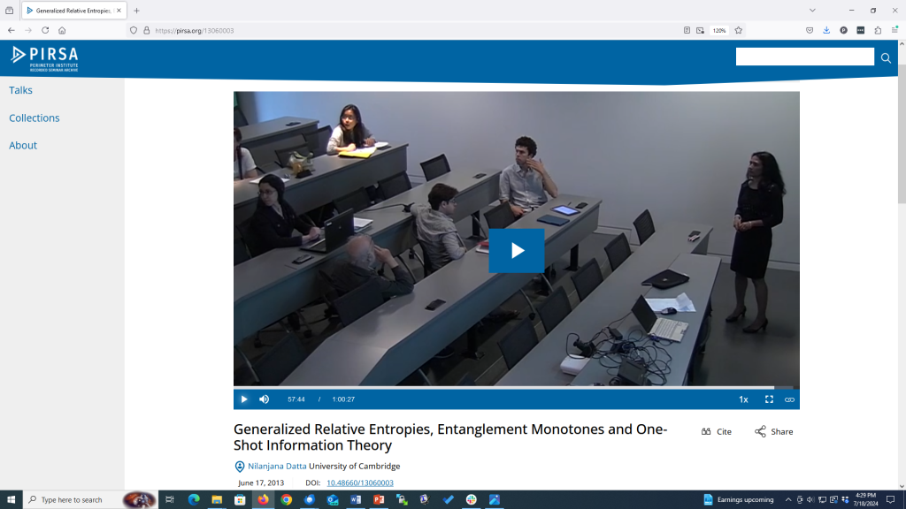
Kudos to John Preskill for hunting down this screenshot of the video of Nilanjana’s seminar. The author appears on the left.

Then, because she eats seminars for breakfast, Nilanjana presented an even more distinguished talk the same day: a colloquium. It took place at the University of Waterloo’s Institute for Quantum Computing (IQC), a nearly half-hour walk from Perimeter. Would I be willing to escort Nilanjana between the two institutes? I most certainly would.

Nilanjana and I arrived at the IQC auditorium before anyone else except the colloquium’s host, Debbie Leung. Debbie is a University of Waterloo professor and another of the most rigorous quantum information theorists I know. I sat a little behind the two of them and marveled. Here were two of the scions of the science I was joining. Pinch me.

My relationship with Nilanjana deepened over the years. The first year of my PhD, she hosted a seminar by me at the University of Cambridge (although I didn’t present a colloquium later that day). Afterward, I wrote a Quantum Frontiers post about her research with PhD student Felix Leditzky. The two of them introduced me to second-order asymptotics. Second-order asymptotics dictate the rate at which one-shot entropies approach standard entropies as n (the number of copies of a message I’m compressing, say) grows large. 

The following year, Nilanjana and colleagues hosted me at “Beyond i.i.d. in Information Theory,” an annual conference dedicated to one-shot information theory. We convened in the mountains of Banff, Canada, about which I wrote another blog post. Come to think of it, Nilanjana lies behind many of my blog posts, as she lies behind many of my papers.

But I haven’t explained about the little black dress. Nilanjana wore one when presenting at Perimeter and the IQC. That year, I concluded that pants and shorts caused me so much discomfort, I’d wear only skirts and dresses. So I stuck out in physics gatherings like a theorem in a newspaper. My mother had schooled me in the historical and socioeconomic significance of the little black dress. Coco Chanel invented the slim, simple, elegant dress style during the 1920s. It helped free women from stifling, time-consuming petticoats and corsets: a few decades beforehand, dressing could last much of the morning—and then one would change clothes for the afternoon and then for the evening. The little black dress offered women freedom of movement, improved health, and control over their schedules. Better, the little black dress could suit most activities, from office work to dinner with friends.

Yet I didn’t recall ever having seen anyone present physics in a little black dress.

I almost never use this verb, but Nilanjana rocked that little black dress. She imbued it with all the professionalism and competence ever associated with it. Also, Nilanjana had long, dark hair, like mine (although I’ve never achieved her hair’s length); and she wore it loose, as I liked to. I recall admiring the hair hanging down her back after she received a question during the IQC colloquium. She’d whirled around to write the answer on the board, in the rapid-fire manner characteristic of her intellect. If one of the most incisive scientists I knew could wear dresses and long hair, then so could I.

Felix is now an assistant professor at the University of Illinois in Urbana-Champaign. I recently spoke with him and Mark Wilde, another one-shot information theorist and a guest blogger on Quantum Frontiers. The conversation led me to reminisce about the day I met Nilanjana. I haven’t visited Cambridge in years, and my research has expanded from one-shot thermodynamics into many-body physics. But one never forgets the classics.


Let gravity do its work

One day, early this spring, I found myself in a hotel elevator with three other people. The cohort consisted of two theoretical physicists, one computer scientist, and what appeared to be a normal person. I pressed the elevator’s 4 button, as my husband (the computer scientist) and I were staying on the hotel’s fourth floor. The button refused to light up.

“That happened last time,” the normal person remarked. He was staying on the fourth floor, too.

The other theoretical physicist pressed the 3 button.

“Should we press the 5 button,” the normal person continued, “and let gravity do its work?

I took a moment to realize that he was suggesting we ascend to the fifth floor and then induce the elevator to fall under gravity’s influence to the fourth. We were reaching floor three, so I exchanged a “have a good evening” with the other physicist, who left. The door shut, and we began to ascend.

As it happens,” I remarked, “he’s an expert on gravity.” The other physicist was Herman Verlinde, a professor at Princeton.

Such is a side effect of visiting the Simons Center for Geometry and Physics. The Simons Center graces the Stony Brook University campus, which was awash in daffodils and magnolia blossoms last month. The Simons Center derives its name from hedge-fund manager Jim Simons (who passed away during the writing of this article). He achieved landmark physics and math research before earning his fortune on Wall Street as a quant. Simons supported his early loves by funding the Simons Center and other scientific initiatives. The center reminded me of the Perimeter Institute for Theoretical Physics, down to the café’s linen napkins, so I felt at home.
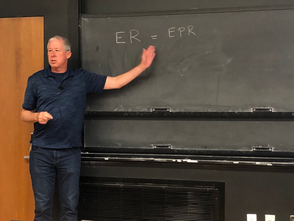
I was participating in the Simons Center workshop “Entanglement, thermalization, and holography.” It united researchers from quantum information and computation, black-hole physics and string theory, quantum thermodynamics and many-body physics, and nuclear physics. We were to share our fields’ approaches to problems centered on thermalization, entanglement, quantum simulation, and the like. I presented about the eigenstate thermalization hypothesis, which elucidates how many-particle quantum systems thermalize. The hypothesis fails, I argued, if a system’s dynamics conserve quantities (analogous to energy and particle number) that can’t be measured simultaneously. Herman Verlinde discussed the ER=EPR conjecture.
My PhD advisor, John Preskill, blogged about ER=EPR almost exactly eleven years ago. Read his blog post for a detailed introduction. Briefly, ER=EPR posits an equivalence between wormholes and entanglement. 

The ER stands for Einstein–Rosen, as in Einstein–Rosen bridge. Sean Carroll provided the punchiest explanation I’ve heard of Einstein–Rosen bridges. He served as the scientific advisor for the 2011 film Thor. Sean suggested that the film feature a wormhole, a connection between two black holes. The filmmakers replied that wormholes were passé. So Sean suggested that the film feature an Einstein–Rosen bridge. “What’s an Einstein–Rosen bridge?” the filmmakers asked. “A wormhole.” So Thor features an Einstein–Rosen bridge.

EPR stands for Einstein–Podolsky–Rosen. The three authors published a quantum paradox in 1935. Their EPR paper galvanized the community’s understanding of entanglement.

ER=EPR is a conjecture that entanglement is closely related to wormholes. As Herman said during his talk, “You probably need entanglement to realize a wormhole.” Or any two maximally entangled particles are connected by a wormhole. The idea crystallized in a paper by Juan Maldacena and Lenny Susskind. They drew on work by Mark Van Raamsdonk (who masterminded the workshop behind this Quantum Frontiers post) and Brian Swingle (who’s appeared in further posts).

Herman presented four pieces of evidence for the conjecture, as you can hear in the video of his talk. One piece emerges from the AdS/CFT duality, a parallel between certain space-times (called anti–de Sitter, or AdS, spaces) and quantum theories that have a certain symmetry (called conformal field theories, or CFTs). A CFT, being quantum, can contain entanglement. One entangled state is called the thermofield double. Suppose that a quantum system is in a thermofield double and you discard half the system. The remaining half looks thermal—we can attribute a temperature to it. Evidence indicates that, if a CFT has a temperature, then it parallels an AdS space that contains a black hole. So entanglement appears connected to black holes via thermality and temperature.

Despite the evidence—and despite the eleven years since John’s publication of his blog post—ER=EPR remains a conjecture. Herman remarked, “It’s more like a slogan than anything else.” His talk’s abstract contains more hedging than a suburban yard. I appreciated the conscientiousness, a college acquaintance having once observed that I spoke carefully even over sandwiches with a friend.

A “source of uneasiness” about ER=EPR, to Herman, is measurability. We can’t check whether a quantum state is entangled via any single measurement. We have to prepare many identical copies of the state, measure the copies, and process the outcome statistics. In contrast, we seem able to conclude that a space-time is connected without measuring multiple copies of the space-time. We can check that a hotel’s first floor is connected to its fourth, for instance, by riding in an elevator once.
Or by riding an elevator to the fifth floor and descending by one story. My husband, the normal person, and I took the stairs instead of falling. The hotel fixed the elevator within a day or two, but who knows when we’ll fix on the truth value of ER=EPR?

With thanks to the conference organizers for their invitation, to the Simons Center for its hospitality, to Jim Simons for his generosity, and to the normal person for inspiration.

You can win Tic Tac Toe, if you know quantum physics.
Note: Oliver Zheng is a senior at University High School, Irvine CA. He has been working on AI players for quantum versions of Tic Tac Toe under the supervision of Dr. Spiros Michalakis.
Several years ago, while scrolling through YouTube, I came across a video of Paul Rudd playing something called “Quantum Chess.” I had no idea what it was, nor did I know that it would become one of the most gloriously nerdy rabbit holes I would ever fall into (see: 5D Chess with Multiverse Time Travel).

Over time, I tried to teach myself how to play these multi-layered, multi-dimensional games, but progress was slow. However, while taking a break during a piano lesson last year, I mentioned to my teacher my growing interest in unnecessarily stressful versions of chess. She told me that she happened to be friends with Dr. Xie Chen, professor of theoretical physics at Caltech who was sponsoring a Quantum Gaming project. I immediately jumped at the opportunity to connect with her, and within days was able to have my first online meeting with Dr. Chen. Soon after, I got invited to join the project. Following my introduction to the team, I started reading “Quantum Computation and Quantum Information”, which helped me understand how the theory behind the games worked. When I felt ready, Dr. Chen referred me to Dr. Spiros Michalakis at Caltech, who, funnily enough, was the creator of the quantum chess video. 

I would’ve never imagined that I am two degrees of separation from Paul Rudd, but nonetheless, I wanted to share some of the work I’ve been doing with Spiros on Quantum TiqTaqToe.

What is Quantum TiqTaqToe?

Evert van Nieuwenburg, the creator of Quantum TiqTaqToe whom I also collaborated with, goes in depth about how the game works here, but I will give a short rundown. The general idea is that there is now a split move, where you can put an ‘X’ in two different squares at once — a Schrödinger’s X, if you will. When the board has no more empty squares, the X randomly ‘collapses’ into one of the two squares with equal probability. The game ends when there are three real X’s or three real O’s in a row, just as in regular tic-tac-toe. Depending on the mode you are playing, you might also be able to entangle your X’s with your opponent’s O’s. You can get a better sense of all this by actually playing the game here.

My goal was to find out who wins when both players play optimally. For instance, in normal tic-tac-toe, it is well-known that the first X should go in the middle of the board, and if player O counters successfully, the game should end in a tie. Is the outcome of Quantum TiqTaqToe, too, predetermined to end in a tie if both players play optimally? And, if not, what is the best first move for player X? I sought to answer these questions through the power of computation.

The First Attempt

In the following section, I refer to a ‘game state’ as any unique arrangement of X’s and O’s on a board. The ‘empty game state’ simply means an empty board. ‘Traversing’ through a certain game state means that, at some point in the game, that game state occurs. So, for example, every game traverses through the empty game state, since every game starts with an empty board.

In order to solve the unsolved, one must first solve the solved. As such, my first attempt was to create an algorithm that would figure out the best move to play in regular tic-tac-toe. This first attempt was rather straightforward, and I will explain it here:

Essentially, I developed a model using what is known as “reinforcement learning” to determine the best next move given a certain game state. Here is how it works: To track which set of moves are best for player X and player O, respectively, every game state is assigned a value, initially 0. When a game ends, these values are updated to reflect who won. The more games are played, the better these values reflect the sequence of moves that X and O must make to win or tie. To train this model (machine learning parlance for the algorithm that updates the values/parameters mentioned above), I programmed the computer to play randomly chosen moves for X and O, until the game ended. If, say, player X won, then the value of every game state traversed was increased by 1 to indicate that X was favored. On the other hand, if player O won, then the value of every game state traversed was decreased by 1 to indicate that O was favored. Here is an example:

X wins!

Let’s say that this is the first iteration that the model is trained on. Then, the next time the model sees this game state,

it will recognize that X has an advantage. In the same vein, the model now also thinks that the empty game state is favorable towards X, since, in the one game that was played, when the empty game state was traversed, X won.

If we run these randomized games enough times (I ran ten million iterations), every move in every game state has most likely been made, which means that the model is able to give a meaningful evaluation for any game state. However, there is one major problem with this approach, in that the model only indicates who is favored when they make a random move, not when they make the best move. To illustrate this, let’s examine the following game state:

(O’s turn)

Here, player O has two options: they can win the game by putting their O on the bottom center square, or lose the game by putting it on the right center square. Any seasoned tic-tac-toe player would make the right move in this scenario, and win the game. However, since the model trains on random moves, it thinks that player O will win half the time and lose half the time. Thus, to the model, this game state is not favorable to either player, when in reality it is absolutely favored towards O. 

During my first meeting with Spiros and Evert, they pointed out this flaw in my model. Evert suggested that I study up on something called a minimax algorithm, which circumvents this flaw, and apply it to tic-tac-toe. This set me on the next step of my journey.

Enter Minimax

The content of this section takes inspiration from this article.

In the minimax algorithm, the two players are known as the ‘maximizer’ and the ‘minimizer’. In the case of tic-tac-toe, X would be the maximizer and O the minimizer. The maximizer’s goal is to maximize their score, while the minimizer’s goal is to minimize their score. In tic-tac-toe, the minimax algorithm is implemented so that a win by X is a score of +1, a win by O is a score of -1, and a tie is simply 0. So X, seeking to maximize their score, would want to win, which makes sense.

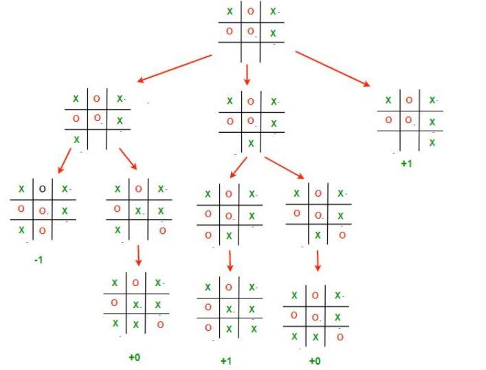
Now, if X wanted to maximize their score through some move, they would have to consider O’s move, who would try to minimize the score. But before O makes their move, they would have to consider X’s next move. This creates a sort of back-and-forth, recursive dynamic in the minimax algorithm. In order for either player to make the best move, they would have to go through all possible moves they can make, and all possible moves their opponent can make after that, and so on and so forth. Here is a relatively simple example of the minimax algorithm at work:

Let’s start from the top. X has three possible moves they can make, and evaluates each of them. 

In the leftmost branch, the result is either -1 or 0, but which is the real score? Well, we expect O to make their best move, and since they are trying to minimize the score, we expect them to choose the ‘-1’ case. So we can say that this move results in a score of -1. 

In the middle branch, the result is either 1 or 0, and, following the same reasoning as before, O chooses the move corresponding to the minimal score, resulting in a score of 0.

Finally, the last branch results in X winning, so the score is +1.

Now, X can finally choose their best move, and in the interest of maximizing the score, places their X on the bottom right square. Intuitively, this makes sense because it was the only move that wins the game for X outright.

Great, but what would a minimax algorithm look like in Quantum Tiqtaqtoe?

Enter Expecti-Minimax

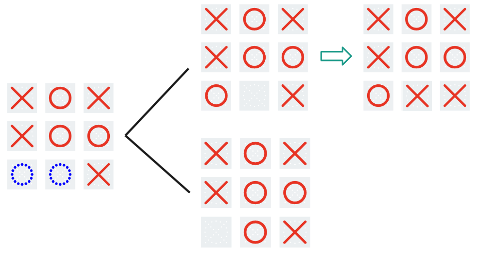
Expectiminimax contains the same core idea as minimax, but something interesting happens when the game board collapses. The algorithm can’t know for sure what the board will look like after collapse, so all it can do is calculate an expected value of the result (hence the name). Let’s look at an example:

Here, collapse occurs, and one branch (top) results in a tie, while the other (bottom) results in O winning. Since a tie is equal to 0 and an O win is equal to -1, the algorithm treats the score as

Note: the sum is divided by two because both outcomes have a ½ probability of occurring.

Solving the Game

Using the expecti-minimax algorithm, I effectively ‘solved’ the minimal and moderate versions of quantum tiqtaqtoe. However, even though the algorithm will always show the best move, the outcome from game to game might not be the same due to the inherent element of randomness. The most interesting of all my discoveries was probably the first move that the algorithm suggests for X, which I was able to make sense of both intuitively and logically. I challenge you all to find it! (Hint: it is the same for both the minimal and moderate versions.)

It turns out that when X plays optimally, they will always win the minimal version no matter what O plays. Meanwhile, in the moderate version, X will win most of the time, but not all the time. The probability distribution is as follows:

  (Another challenge: why are the denominators powers of two?)

Having satisfied my curiosity (for now), I’m looking forward to creating a new game of my own: 4 by 4 quantum tic-tac-toe. Currently, I am working on an algorithm that will give the best move, but since a 4×4 board is almost two times larger than a 3×3 board, the computational runtime of an expectiminimax algorithm would be far too large. As such, I am exploring the use of heuristics, which is sort of what the human mind uses to approach a game like tic-tac-toe. Because of this reliance on heuristics, there is no longer a guarantee that the algorithm will always make the best move, making this new adventure all the more mysterious and captivating. 

Astrobiology meets quantum computation?

The origin of life appears to share little with quantum computation, apart from the difficulty of achieving it and its potential for clickbait. Yet similar notions of complexity have recently garnered attention in both fields. Each topic’s researchers expect only special systems to generate high values of such complexity, or complexity at high rates: organisms, in one community, and quantum computers (and perhaps black holes), in the other. 

Each community appears fairly unaware of its counterpart. This article is intended to introduce the two. Below, I review assembly theory from origin-of-life studies, followed by quantum complexity. I’ll then compare and contrast the two concepts. Finally, I’ll suggest that origin-of-life scientists can quantize assembly theory using quantum complexity. The idea is a bit crazy, but, well, so what?

Assembly theory in origin-of-life studies

Imagine discovering evidence of extraterrestrial life. How could you tell that you’d found it? You’d have detected a bunch of matter—a bunch of particles, perhaps molecules. What about those particles could evidence life?

This question motivated Sara Imari Walker and Lee Cronin to develop assembly theory. (Most of my assembly-theory knowledge comes from Sara, about whom I wrote this blog post years ago and with whom I share a mentor.) Assembly theory governs physical objects, from proteins to self-driving cars. 

Imagine assembling a protein from its constituent atoms. First, you’d bind two atoms together. Then, you might bind another two atoms together. Eventually, you’d bind two pairs together. Your sequence of steps would form an algorithm for assembling the protein. Many algorithms can generate the same protein. One algorithm has the least number of steps. That number is called the protein’s assembly number.

Different natural processes tend to create objects that have different assembly numbers. Stars form low-assembly-number objects by fusing two hydrogen atoms together into helium. Similarly, random processes have high probabilities of forming low-assembly-number objects. For example, geological upheavals can bring a shard of iron near a lodestone. The iron will stick to the magnetized stone, forming a two-component object.

My laptop has an enormous assembly number. Why can such an object exist? Because of information, Sara and Lee emphasize. Human beings amassed information about materials science, Boolean logic, the principles of engineering, and more. That information—which exists only because organisms exists—helped engender my laptop.

If any object has a high enough assembly number, Sara and Lee posit, that object evidences life. Absent life, natural processes have too low a probability of randomly throwing together molecules into the shape of a computer. How high is “high enough”? Approximately fifteen, experiments by Lee’s group suggest. (Why do those experiments point to the number fifteen? Sara’s group is working on a theory for predicting the number.)

In summary, assembly number quantifies complexity in origin-of-life studies, according to Sara and Lee. The researchers propose that only living beings create high-assembly-number objects.

Quantum complexity in quantum computation

Quantum complexity defines a stage in the equilibration of many-particle quantum systems. Consider a clump of N quantum particles isolated from its environment. The clump will be in a pure quantum state | \psi(0) \rangle at a time t = 0. The particles will interact, evolving the clump’s state as a function  | \psi(t) \rangle

Quantum many-body equilibration is more complicated than the equilibration undergone by your afternoon pick-me-up as it cools.

The interactions will equilibrate the clump internally. One stage of equilibration centers on local observables O. They’ll come to have expectation values \langle \psi(t) | O | \psi(t) \rangle approximately equal to thermal expectation values {\rm Tr} ( O \, \rho_{\rm th} ), for a thermal state \rho_{\rm th} of the clump. During another stage of equilibration, the particles correlate through many-body entanglement. 

The longest known stage centers on the quantum complexity of | \psi(t) \rangle. The quantum complexity is the minimal number of basic operations needed to prepare | \psi(t) \rangle from a simple initial state. We can define “basic operations” in many ways. Examples include quantum logic gates that act on two particles. Another example is an evolution for one time step under a Hamiltonian that couples together at most k particles, for some k independent of N. Similarly, we can define “a simple initial state” in many ways. We could count as simple only the N-fold tensor product | 0 \rangle^{\otimes N} of our favorite single-particle state | 0 \rangle. Or we could call any N-fold tensor product simple, or any state that contains at-most-two-body entanglement, and so on. These choices don’t affect the quantum complexity’s qualitative behavior, according to string theorists Adam Brown and Lenny Susskind.

How quickly can the quantum complexity of | \psi(t) \rangle grow? Fast growth stems from many-body interactions, long-range interactions, and random coherent evolutions. (Random unitary circuits exemplify random coherent evolutions: each gate is chosen according to the Haar measure, which we can view roughly as uniformly random.) At most, quantum complexity can grow linearly in time. Random unitary circuits achieve this rate. Black holes may; they scramble information quickly. The greatest possible complexity of any N-particle state scales exponentially in N, according to a counting argument

A highly complex state | \psi(t) \rangle looks simple from one perspective and complicated from another. Human scientists can easily measure only local observables O. Such observables’ expectation values \langle \psi(t) | O | \psi(t) \rangle  tend to look thermal in highly complex states, \langle \psi(t) | O | \psi(t) \rangle \approx {\rm Tr} ( O \, \rho_{\rm th} ), as implied above. The thermal state has the greatest von Neumann entropy, - {\rm Tr} ( \rho \log \rho), of any quantum state \rho that obeys the same linear constraints as | \psi(t) \rangle (such as having the same energy expectation value). Probed through simple, local observables O, highly complex states look highly entropic—highly random—similarly to a flipped coin.

Yet complex states differ from flipped coins significantly, as revealed by subtler analyses. An example underlies the quantum-supremacy experiment published by Google’s quantum-computing group in 2018. Experimentalists initialized 53 qubits (quantum two-level systems) in a tensor product. The state underwent many gates, which prepared a highly complex state. Then, the experimentalists measured the z-component \sigma_z of each qubit’s spin, randomly obtaining a -1 or a 1. One trial yielded a 53-bit string. The experimentalists repeated this process many times, using the same gates in each trial. From all the trials’ bit strings, the group inferred the probability p(s) of obtaining a given string s in the next trial. The distribution \{ p(s) \} resembles the uniformly random distribution…but differs from it subtly, as revealed by a cross-entropy analysis. Classical computers can’t easily generate \{ p(s) \}; hence the Google group’s claiming to have achieved quantum supremacy/advantage. Quantum complexity differs from simple randomness, that difference is difficult to detect, and the difference can evidence quantum computers’ power.

A fridge that holds one of Google’s quantum computers.

Comparison and contrast

Assembly number and quantum complexity resemble each other as follows:

  1. Each function quantifies the fewest basic operations needed to prepare something.
  2. Only special systems (organisms) can generate high assembly numbers, according to Sara and Lee. Similarly, only special systems (such as quantum computers and perhaps black holes) can generate high complexity quickly, quantum physicists expect.
  3. Assembly number may distinguish products of life from products of abiotic systems. Similarly, quantum complexity helps distinguish quantum computers’ computational power from classical computers’.
  4. High-assembly-number objects are highly structured (think of my laptop). Similarly, high-complexity quantum states are highly structured in the sense of having much many-body entanglement.
  5. Organisms generate high assembly numbers, using information. Similarly, using information, organisms have created quantum computers, which can generate quantum complexity quickly.

Assembly number and quantum complexity differ as follows:

  1. Classical objects have assembly numbers, whereas quantum states have quantum complexities.
  2. In the absence of life, random natural processes have low probabilities of producing high-assembly-number objects. That is, randomness appears to keep assembly numbers low. In contrast, randomness can help quantum complexity grow quickly.
  3. Highly complex quantum states look very random, according to simple, local probes. High-assembly-number objects do not.
  4. Only organisms generate high assembly numbers, according to Sara and Lee. In contrast, abiotic black holes may generate quantum complexity quickly.

Another feature shared by assembly-number studies and quantum computation merits its own paragraph: the importance of robustness. Suppose that multiple copies of a high-assembly-number (or moderate-assembly-number) object exist. Not only does my laptop exist, for example, but so do many other laptops. To Sara, such multiplicity signals the existence of some stable mechanism for creating that object. The multiplicity may provide extra evidence for life (including life that’s discovered manufacturing), as opposed to an unlikely sequence of random forces. Similarly, quantum computing—the preparation of highly complex states—requires stability. Decoherence threatens quantum states, necessitating quantum error correction. Quantum error correction differs from Sara’s stable production mechanism, but both evidence the importance of robustness to their respective fields.

A modest proposal

One can generalize assembly number to quantum states, using quantum complexity. Imagine finding a clump of atoms while searching for extraterrestrial life. The atoms need not have formed molecules, so the clump can have a low classical assembly number. However, the clump can be in a highly complex quantum state. We could detect the state’s complexity only (as far as I know) using many copies of the state, so imagine finding many clumps of atoms. Preparing highly complex quantum states requires special conditions, such as a quantum computer. The clump might therefore evidence organisms who’ve discovered quantum physics. Using quantum complexity, one might extend the assembly number to identify quantum states that may evidence life. However, quantum complexity, or a high rate of complexity generation, alone may not evidence life—for example, if achievable by black holes. Fortunately, a black hole seems unlikely to generate many identical copies of a highly complex quantum state. So we seem to have a low probability of mistakenly attributing a highly complex quantum state, sourced by a black hole, to organisms (atop our low probability of detecting any complex quantum state prepared by anyone other than us).

Would I expect a quantum assembly number to greatly improve humanity’s search for extraterrestrial life? I’m no astrobiology expert (NASA videos notwithstanding), but I’d expect probably not. Still, astrobiology requires chemistry, which requires quantum physics. Quantum complexity seems likely to find applications in the assembly-number sphere. Besides, doesn’t juxtaposing the search for extraterrestrial life and the understanding of life’s origins with quantum computing sound like fun? And a sense of fun distinguishes certain living beings from inanimate matter about as straightforwardly as assembly number does.

With thanks to Jim Al-Khalili, Paul Davies, the From Physics to Life collaboration, and UCLA for hosting me at the workshop that spurred this article.

Can Thermodynamics Resolve the Measurement Problem?

At the recent Quantum Thermodynamics conference in Vienna (coming next year to the University of Maryland!), during an expert panel Q&A session, one member of the audience asked “can quantum thermodynamics address foundational problems in quantum theory?”

That stuck with me, because that’s exactly what my research is about. So naturally, I’d say the answer is yes! In fact, here in the group of Marcus Huber at the Technical University of Vienna, we think thermodynamics may have something to say about the biggest quantum foundations problem of all: the measurement problem.

It’s sort of the iconic mystery of quantum mechanics: we know that an electron can be in two places at once – in a ‘superposition’ – but when we measure it, it’s only ever seen to be in one place, picked seemingly at random from the two possibilities. We say the state has ‘collapsed’.

What’s going on here? Thanks to Bell’s legendary theorem, we know that the answer can’t just be that it was always actually in one place and we just didn’t know which option it was – it really was in two places at once until it was measured1. But also, we don’t see this effect for sufficiently large objects. So how can this ‘two-places-at-once’ thing happen at all, and why does it stop happening once an object gets big enough?

Here, we already see hints that thermodynamics is involved, because even classical thermodynamics says that big systems behave differently from small ones. And interestingly, thermodynamics also hints that the narrative so far can’t be right. Because when taken at face value, the ‘collapse’ model of measurement breaks all three laws of thermodynamics.

Imagine an electron in a superposition of two energy levels: a combination of being in its ground state and first excited state. If we measure it and it ‘collapses’ to being only in the ground state, then its energy has decreased: it went from having some average of the ground and excited energies to just having the ground energy. The first law of thermodynamics says (crudely) that energy is conserved, but the loss of energy is unaccounted for here.

Next, the second law says that entropy always increases. One form of entropy represents your lack of information about a system’s state. Before the measurement, the system was in one of two possible states, but afterwards it was in only one state. So speaking very broadly, our uncertainty about its state, and hence the entropy, is reduced. (The third law is problematic here, too.)

There’s a clear explanation here: while the system on its own decreases its entropy and doesn’t conserve energy, in order to measure something, we must couple the system to a measuring device. That device’s energy and entropy changes must account for the system’s changes.

This is the spirit of our measurement model2. We explicitly include the detector as a quantum object in the record-keeping of energy and information flow. In fact, we also include the entire environment surrounding both system and device – all the lab’s stray air molecules, photons, etc. Then the idea is to describe a measurement process as propagating a record of a quantum system’s state into the surroundings without collapsing it.

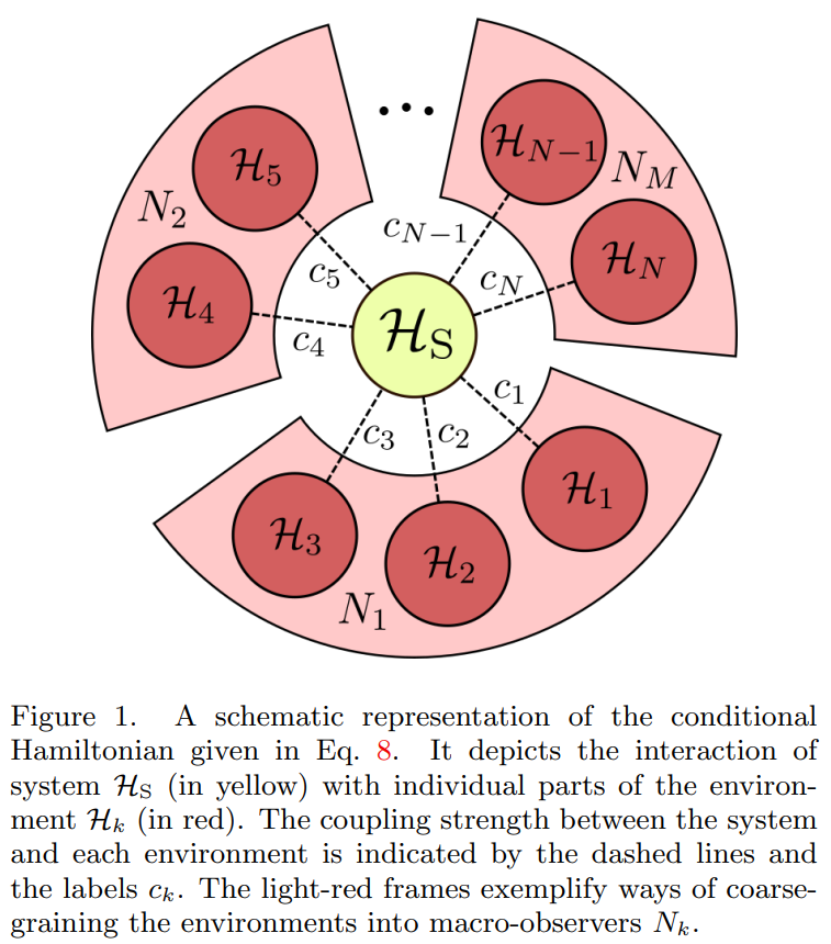
A schematic representation of a system spreading information into an environment (from Schwarzhans et al., with permission)

But talking about quantum systems interacting with their environments is nothing new. The “decoherence” model from the 70s, which our work builds on, says quantum objects become less quantum when buffeted by a larger environment.

The problem, though, is that decoherence describes how information is lost into an environment, and so usually the environment’s dynamics aren’t explicitly calculated: this is called an open-system approach. By contrast, in the closed-system approach we use, you model the dynamics of the environment too, keeping track of all information. This is useful because conventional collapse dynamics seems to destroy information, but every other fundamental law of physics seems to say that information can’t be destroyed.

This all allows us to track how information flows from system to surroundings, using the “Quantum Darwinism” (QD) model of W.H. Żurek. Whereas decoherence describes how environments affect systems, QD describes how quantum systems impact their environments by spreading information into them. The QD model says that the most ‘classical’ information – the kind most consistent with classical notions of ‘being in one place’, etc. – is the sort most likely to ‘survive’ the decoherence process.

QD then further asserts that this is the information that’s most likely to be copied into the environment. If you look at some of a system’s surroundings, this is what you’d most likely see. (The ‘Darwinism’ name is because certain states are ‘selected for’ and ‘replicate’3.)

So we have a description of what we want the post-measurement state to look like: a decohered system, with its information redundantly copied into its surrounding environment. The last piece of the puzzle, then, is to ask how a measurement can create this state. Here, we finally get to the dynamics part of the thermodynamics, and introduce equilibration.

Earlier we said that even if the system’s entropy decreases, the detector’s entropy (or more broadly the environment’s) should go up to compensate. Well, equilibration maximizes entropy. In particular, equilibration describes how a system tends towards a particular ‘equilibrium’ state, because the system can always increase its entropy by getting closer to it.

It’s usually said that systems equilibrate if put in contact with an external environment (e.g. a can of beer cooling in a fridge), but we’re actually interested in a different type of equilibration called equilibration on average. There, we’re asking for the state that a system stays roughly close to, on average, over long enough times, with no outside contact. That means it never actually decoheres, it just looks like it does for certain observables. (This actually implies that nothing ever actually decoheres, since open systems are only an approximation you make when you don’t want to track all of the environment.)

Equilibration is the key to the model. In fact, we call our idea the Measurement-Equilibration Hypothesis (MEH): we’re asserting that measurement is an equilibration process. Which makes the final question: what does all this mean for the measurement problem?

In the MEH framework, when someone ‘measures’ a quantum system, they allow some measuring device, plus a chaotic surrounding environment, to interact with it. The quantum system then equilibrates ‘on average’ with the environment, and spreads information about its classical states into the surroundings. Since you are a macroscopically large human, any measurement you do will induce this sort of equilibration to happen, meaning you will only ever have access to the classical information in the environment, and never see superpositions. But no collapse is necessary, and no information is lost: rather some information is only much more difficult to access in all the environment noise, as happens all the time in the classical world.

It’s tempting to ask what ‘happens’ to the outcomes we don’t see, and how nature ‘decides’ which outcome to show to us. Those are great questions, but in our view, they’re best left to philosophers4. For the question we care about: why measurements look like a ‘collapse’, we’re just getting started with our Measurement-Equilibration Hypothesis – there’s still lots to do in our explorations of it. We think the answers we’ll uncover in doing so will form an exciting step forward in our understanding of the weird and wonderful quantum world.

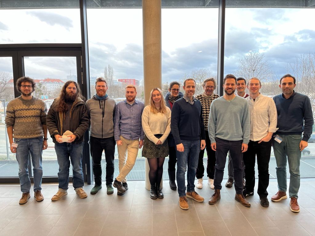
Members of the MEH team at a kick-off meeting for the project in Vienna in February 2023. Left to right: Alessandro Candeloro, Marcus Huber, Emanuel Schwarzhans, Tom Rivlin, Sophie Engineer, Veronika Baumann, Nicolai Friis, Felix C. Binder, Mehul Malik, Maximilian P.E. Lock, Pharnam Bakhshinezhad

Acknowledgements: Big thanks to the rest of the MEH team for all the help and support, in particular Dr. Emanuel Schwarzhans and Dr. Lock for reading over this piece!)

Here are a few choice references (by no means meant to be comprehensive!)

Quantum Thermodynamics (QTD) Conference 2023: https://qtd2023.conf.tuwien.ac.at/
QTD 2024: https://qtd-hub.umd.edu/event/qtd-conference-2024/
Bell’s Theorem: https://plato.stanford.edu/entries/bell-theorem/
The first MEH paper: https://arxiv.org/abs/2302.11253
A review of decoherence: https://journals.aps.org/rmp/abstract/10.1103/RevModPhys.75.715
Quantum Darwinism: https://www.nature.com/articles/nphys1202
Measurements violate the 3rd law: https://quantum-journal.org/papers/q-2020-01-13-222/
More on the 3rd and QM: https://journals.aps.org/prxquantum/abstract/10.1103/PRXQuantum.4.010332
Equilibration on average: https://iopscience.iop.org/article/10.1088/0034-4885/79/5/056001/meta
Objectivity: https://journals.aps.org/pra/abstract/10.1103/PhysRevA.91.032122

  1. There is a perfectly valid alternative with other weird implications: that it was always just in one place, but the world is intrinsically non-local. Most physicists prefer to save locality over realism, though. ↩︎
  2. First proposed in this paper by Schwarzhans, Binder, Huber, and Lock: https://arxiv.org/abs/2302.11253 ↩︎
  3. In my opinion… it’s a brilliant theory with a terrible name! Sure, there’s something akin to ‘selection pressure’ and ‘reproduction’, but there aren’t really any notions of mutation, adaptation, fitness, generations… Alas, the name has stuck. ↩︎
  4. I actually love thinking about this question, and the interpretations of quantum mechanics more broadly, but it’s fairly orthogonal to the day-to-day research on this model. ↩︎

The Book of Mark, Chapter 2

Late in the summer of 2021, I visited a physics paradise in a physical paradise: the Kavli Institute for Theoretical Physics (KITP). The KITP sits at the edge of the University of California, Santa Barbara like a bougainvillea bush at the edge of a yard. I was eating lunch outside the KITP one afternoon, across the street from the beach. PhD student Arman Babakhani, whom a colleague had just introduced me to, had joined me.

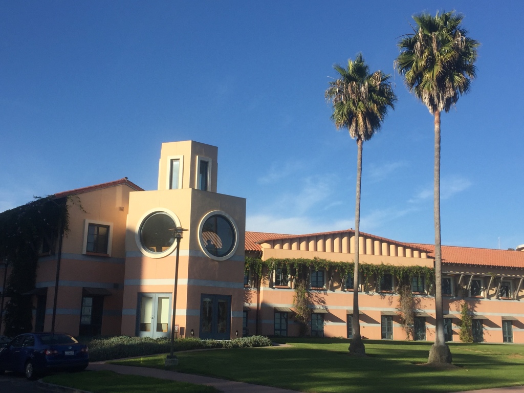
The KITP’s Kohn Hall

What physics was I working on nowadays? Arman wanted to know.

Thermodynamic exchanges. 

The world consists of physical systems exchanging quantities with other systems. When a rose blooms outside the Santa Barbara mission, it exchanges pollen with the surrounding air. The total amount of pollen across the rose-and-air whole remains constant, so we call the amount a conserved quantity. Quantum physicists usually analyze conservation of particles, energy, and magnetization. But quantum systems can conserve quantities that participate in uncertainty relations. Such quantities are called incompatible, because you can’t measure them simultaneously. The x-, y-, and z-components of a qubit’s spin are incompatible.

The Santa Barbara mission…
…and its roses

Exchanging and conserving incompatible quantities, systems can violate thermodynamic expectations. If one system is much larger than the other, we expect the smaller system to thermalize; yet incompatibility invalidates derivations of the thermal state’s form. Incompatibility reduces the thermodynamic entropy produced by exchanges. And incompatibility can raise the average amount entanglement in the pair of systems—the total system.

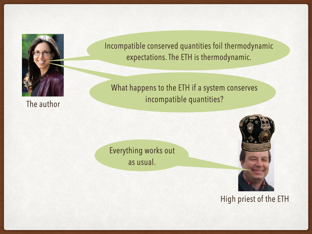
If the total system conserves incompatible quantities, what happens to the eigenstate thermalization hypothesis (ETH)? Last month’s blog post overviewed the ETH, a framework for understanding how quantum many-particle systems thermalize internally. That post labeled Mark Srednicki, a professor at the KITP, a high priest of the ETH. I want, I told Arman, to ask Mark what happens when you combine the ETH with incompatible conserved quantities.

I’ll do it, Arman said.

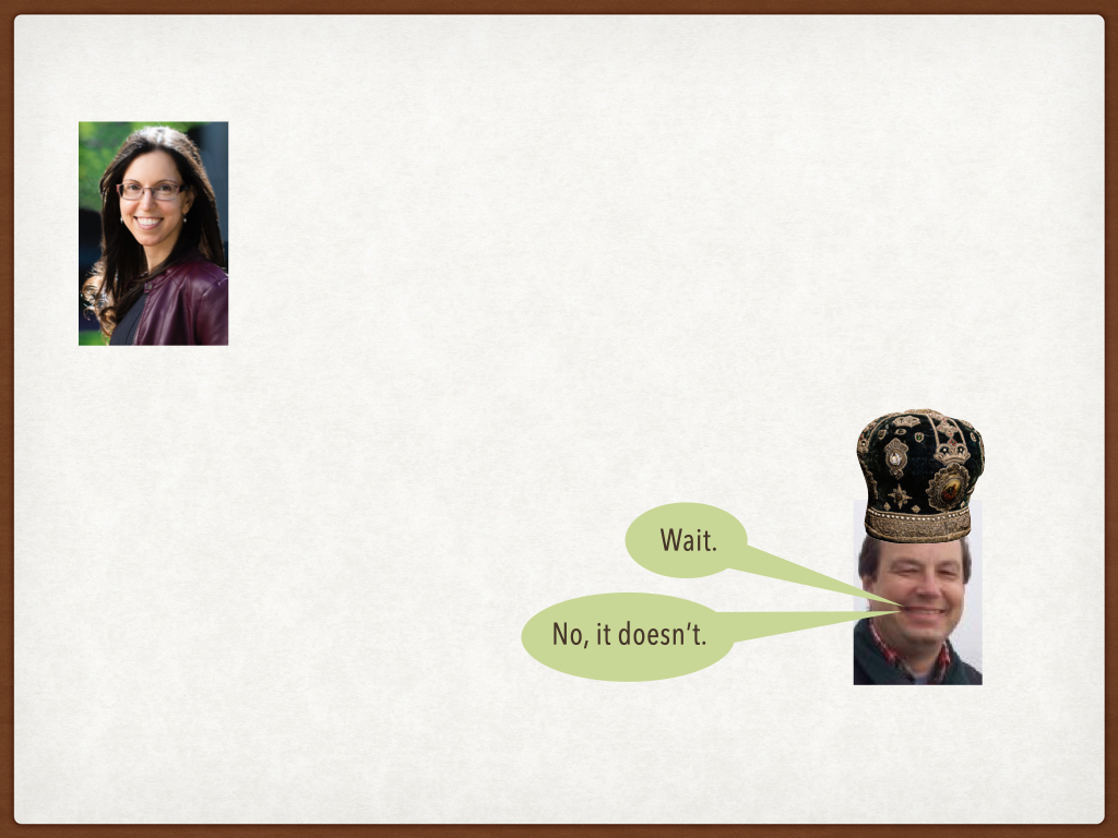
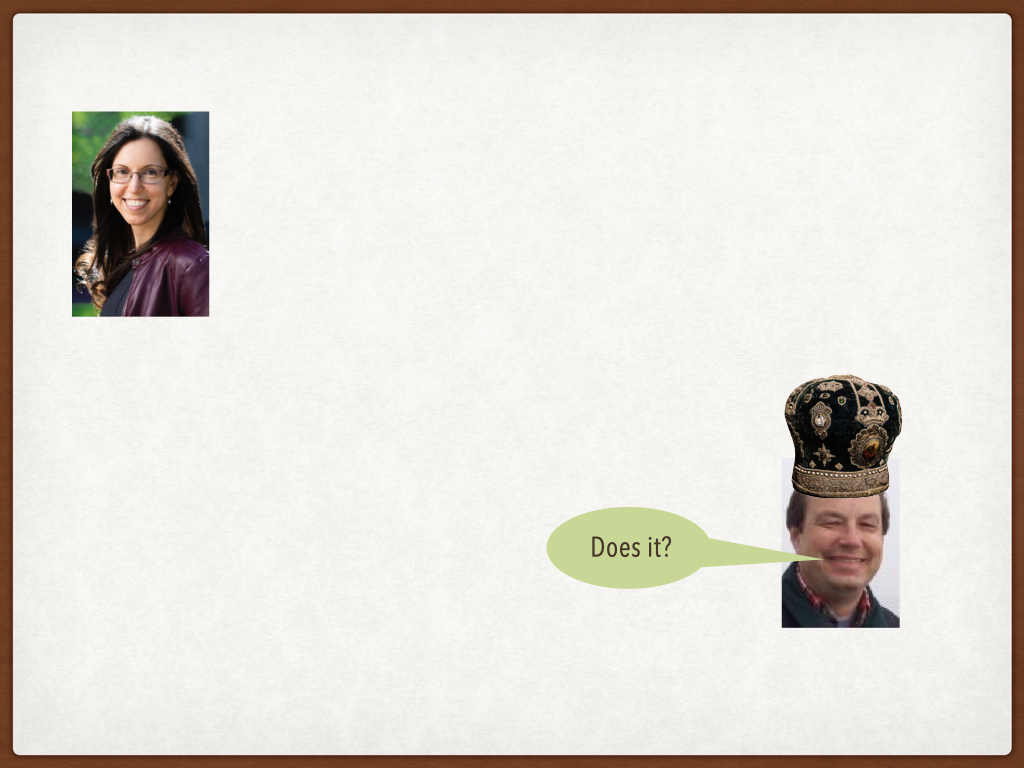
Soon after, I found myself in the fishbowl. High up in the KITP, a room filled with cushy seats overlooks the ocean. The circular windows lend the room its nickname. Arrayed on the armchairs and couches were Mark, Arman, Mark’s PhD student Fernando Iniguez, and Mark’s recent PhD student Chaitanya Murthy. The conversation went like this:

Mark was frustrated about not being able to answer the question. I was delighted to have stumped him. Over the next several weeks, the group continued meeting, and we emailed out notes for everyone to criticize. I particulary enjoyed watching Mark and Chaitanya interact. They’d grown so intellectually close throughout Chaitanya’s PhD studies, they reminded me of an old married couple. One of them had to express only half an idea for the other to realize what he’d meant and to continue the thread. Neither had any qualms with challenging the other, yet they trusted each other’s judgment.1

In vintage KITP fashion, we’d nearly completed a project by the time Chaitanya and I left Santa Barbara. Physical Review Letters published our paper this year, and I’m as proud of it as a gardener of the first buds from her garden. Here’s what we found.

Southern California spoiled me for roses.

Incompatible conserved quantities conflict with the ETH and the ETH’s prediction of internal thermalization. Why? For three reasons. First, when inferring thermalization from the ETH, we assume that the Hamiltonian lacks degeneracies (that no energy equals any other). But incompatible conserved quantities force degeneracies on the Hamiltonian.2 

Second, when inferring from the ETH that the system thermalizes, we assume that the system begins in a microcanonical subspace. That’s an eigenspace shared by the conserved quantities (other than the Hamiltonian)—usually, an eigenspace of the total particle number or the total spin’s z-component. But, if incompatible, the conserved quantities share no eigenbasis, so they might not share eigenspaces, so microcanonical subspaces won’t exist in abundance.

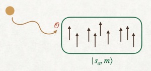
Third, let’s focus on a system of N qubits. Say that the Hamiltonian conserves the total spin components S_x, S_y, and S_z. The Hamiltonian obeys the Wigner–Eckart theorem, which sounds more complicated than it is. Suppose that the qubits begin in a state | s_\alpha, \, m \rangle labeled by a spin quantum number s_\alpha and a magnetic spin quantum number m. Let a particle hit the qubits, acting on them with an operator \mathcal{O} . With what probability (amplitude) do the qubits end up with quantum numbers s_{\alpha'} and m'? The answer is \langle s_{\alpha'}, \, m' | \mathcal{O} | s_\alpha, \, m \rangle. The Wigner–Eckart theorem dictates this probability amplitude’s form. 

| s_\alpha, \, m \rangle and | s_{\alpha'}, \, m' \rangle are Hamiltonian eigenstates, thanks to the conservation law. The ETH is an ansatz for the form of \langle s_{\alpha'}, \, m' | \mathcal{O} | s_\alpha, \, m \rangle—of the elements of matrices that represent operators \mathcal{O} relative to the energy eigenbasis. The ETH butts heads with the Wigner–Eckart theorem, which also predicts the matrix element’s form.

The Wigner–Eckart theorem wins, being a theorem—a proved claim. The ETH is, as the H in the acronym relates, only a hypothesis.

If conserved quantities are incompatible, we have to kiss the ETH and its thermalization predictions goodbye. But must we set ourselves adrift entirely? Can we cling to no buoy from physics’s best toolkit for quantum many-body thermalization?

No, and yes, respectively. Our clan proposed a non-Abelian ETH for Hamiltonians that conserve incompatible quantities—or, equivalently, that have non-Abelian symmetries. The non-Abelian ETH depends on s_\alpha and on Clebsch–Gordan coefficients—conversion factors between total-spin eigenstates | s_\alpha, \, m \rangle and product states | s_1, \, m_1 \rangle \otimes | s_2, \, m_2 \rangle.

Using the non-Abelian ETH, we proved that many systems thermalize internally, despite conserving incompatible quantities. Yet the incompatibility complicates the proof enormously, extending it from half a page to several pages. Also, under certain conditions, incompatible quantities may alter thermalization. According to the conventional ETH, time-averaged expectation values \overline{ \langle \mathcal{O} \rangle }_t come to equal thermal expectation values \langle \mathcal{O} \rangle_{\rm th} to within O( N^{-1} ) corrections, as I explained last month. The correction can grow polynomially larger in the system size, to O( N^{-1/2} ), if conserved quantities are incompatible. Our conclusion holds under an assumption that we argue is physically reasonable.

So incompatible conserved quantities do alter the ETH, yet another thermodynamic expectation. Physicist Jae Dong Noh began checking the non-Abelian ETH numerically, and more testing is underway. And I’m looking forward to returning to the KITP this fall. Tales do say that paradise is a garden.

View through my office window at the KITP

1Not that married people always trust each other’s judgment.

2The reason is Schur’s lemma, a group-theoretic result. Appendix A of this paper explains the details.

The Book of Mark

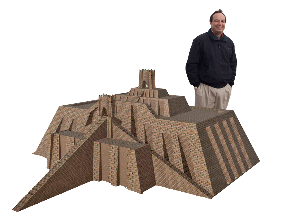
Mark Srednicki doesn’t look like a high priest. He’s a professor of physics at the University of California, Santa Barbara (UCSB); and you’ll sooner find him in khakis than in sacred vestments. Humor suits his round face better than channeling divine wrath would; and I’ve never heard him speak in tongues—although, when an idea excites him, his hands rise to shoulder height of their own accord, as though halfway toward a priestly blessing. Mark belongs less on a ziggurat than in front of a chalkboard. Nevertheless, he called himself a high priest.

Specifically, Mark jokingly called himself a high priest of the eigenstate thermalization hypothesis, a framework for understanding how quantum many-body systems thermalize internally. The eigenstate thermalization hypothesis has an unfortunate number of syllables, so I’ll call it the ETH. The ETH illuminates closed quantum many-body systems, such as a clump of N ultracold atoms. The clump can begin in a pure product state | \psi(0) \rangle, then evolve under a chaotic1 Hamiltonian H. The time-t state | \psi(t) \rangle will remain pure; its von Neumann entropy will always vanish. Yet entropy grows according to the second law of thermodynamics. Breaking the second law amounts almost to a enacting a miracle, according to physicists. Does the clump of atoms deserve consideration for sainthood?

No—although the clump’s state remains pure, a small subsystem’s state does not. A subsystem consists of, for example, a few atoms. They’ll entangle with the other atoms, which serve as an effective environment. The entanglement will mix the few atoms’ state, whose von Neumann entropy will grow.

The ETH predicts this growth. The ETH is an ansatz about H and an operator O—say, an observable of the few-atom subsystem. We can represent O as a matrix relative to the energy eigenbasis. The matrix elements have a certain structure, if O and H satisfy the ETH. Suppose that the operators do and that H lacks degeneracies—that no two energy eigenvalues equal each other. We can prove that O thermalizes: Imagine measuring the expectation value \langle \psi(t) | O | \psi(t) \rangle at each of many instants t. Averaging over instants produces the time-averaged expectation value \overline{ \langle O \rangle_t }

Another average is the thermal average—the expectation value of O in the appropriate thermal state. If H conserves just itself,2 the appropriate thermal state is the canonical state, \rho_{\rm can} := e^{-\beta H}/ Z. The average energy \langle \psi(0) | H | \psi(0) \rangle defines the inverse temperature \beta, and Z normalizes the state. Hence the thermal average is \langle O \rangle_{\rm th}  :=  {\rm Tr} ( O \rho_{\rm can} )

The time average approximately equals the thermal average, according to the ETH: \overline{ \langle O \rangle_t }  =  \langle O \rangle_{\rm th} + O \big( N^{-1} \big). The correction is small in the total number N of atoms. Through the lens of O, the atoms thermalize internally. Local observables tend to satisfy the ETH, and we can easily observe only local observables. We therefore usually observe thermalization, consistently with the second law of thermodynamics.

I agree that Mark Srednicki deserves the title high priest of the ETH. He and Joshua Deutsch independently dreamed up the ETH in 1994 and 1991. Since numericists reexamined it in 2008, studies and applications of the ETH have exploded like a desert religion. Yet Mark had never encountered the question I posed about it in 2021. Next month’s blog post will share the good news about that question.

1Nonintegrable.

2Apart from trivial quantities, such as projectors onto eigenspaces of H.

Let the great world spin

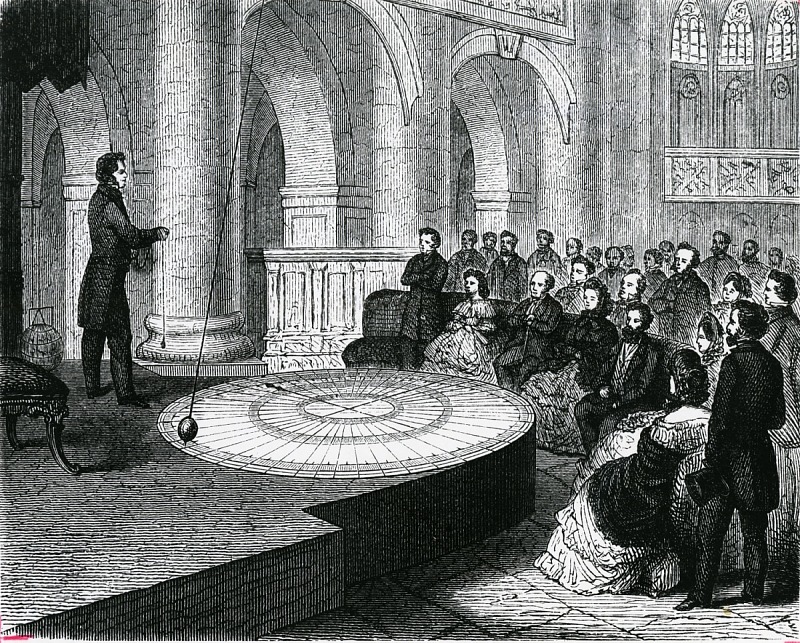
I first heard the song “Fireflies,” by Owl City, shortly after my junior year of college. During the refrain, singer Adam Young almost whispers, “I’d like to make myself believe / that planet Earth turns slowly.” Goosebumps prickled along my neck. Yes, I thought, I’ve studied Foucault’s pendulum.

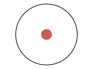
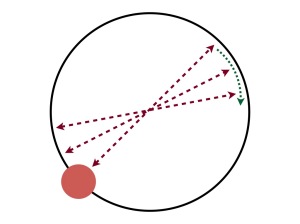
Léon Foucault practiced physics in France during the mid-1800s. During one of his best-known experiments, he hung a pendulum from high up in a building. Imagine drawing a wide circle on the floor, around the pendulum’s bob.1

Pendulum bob and encompassing circle, as viewed from above.

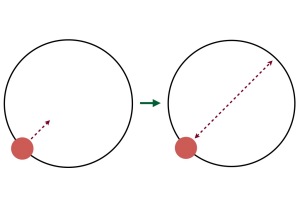
Imagine pulling the bob out to a point above the circle, then releasing the pendulum. The bob will swing back and forth, tracing out a straight line across the circle.

You might expect the bob to keep swinging back and forth along that line, and to do nothing more, forever (or until the pendulum has spent all its energy on pushing air molecules out of its way). After all, the only forces acting on the bob seem to be gravity and the tension in the pendulum’s wire. But the line rotates; its two tips trace out the circle.

How long the tips take to trace the circle depends on your latitude. At the North and South Poles, the tips take one day.

Why does the line rotate? Because the pendulum dangles from a building on the Earth’s surface. As the Earth rotates, so does the building, which pushes the pendulum. You’ve experienced such a pushing if you’ve ridden in a car. Suppose that the car is zipping along at a constant speed, in an unchanging direction, on a smooth road. With your eyes closed, you won’t feel like you’re moving. The only forces you can sense are gravity and the car seat’s preventing you from sinking into the ground (analogous to the wire tension that prevents the pendulum bob from crashing into the floor). If the car turns a bend, it pushes you sidewise in your seat. This push is called a centrifugal force. The pendulum feels a centrifugal force because the Earth’s rotation is an acceleration like the car’s. The pendulum also feels another force—a Coriolis force—because it’s not merely sitting, but moving on the rotating Earth.

We can predict the rotation of Foucault’s pendulum by assuming that the Earth rotates, then calculating the centrifugal and Coriolis forces induced, and then calculating how those forces will influence the pendulum’s motion. The pendulum evidences the Earth’s rotation as nothing else had before debuting in 1851. You can imagine the stir created by the pendulum when Foucault demonstrated it at the Observatoire de Paris and at the Panthéon monument. Copycat pendulums popped up across the world. One ended up next to my college’s physics building, as shown in this video. I reveled in understanding that pendulum’s motion, junior year.

My professor alluded to a grander Foucault pendulum in Paris. It hangs in what sounded like a temple to the Enlightenment—beautiful in form, steeped in history, and rich in scientific significance. I’m a romantic about the Enlightenment; I adore the idea of creating the first large-scale organizational system for knowledge. So I hungered to make a pilgrimage to Paris.

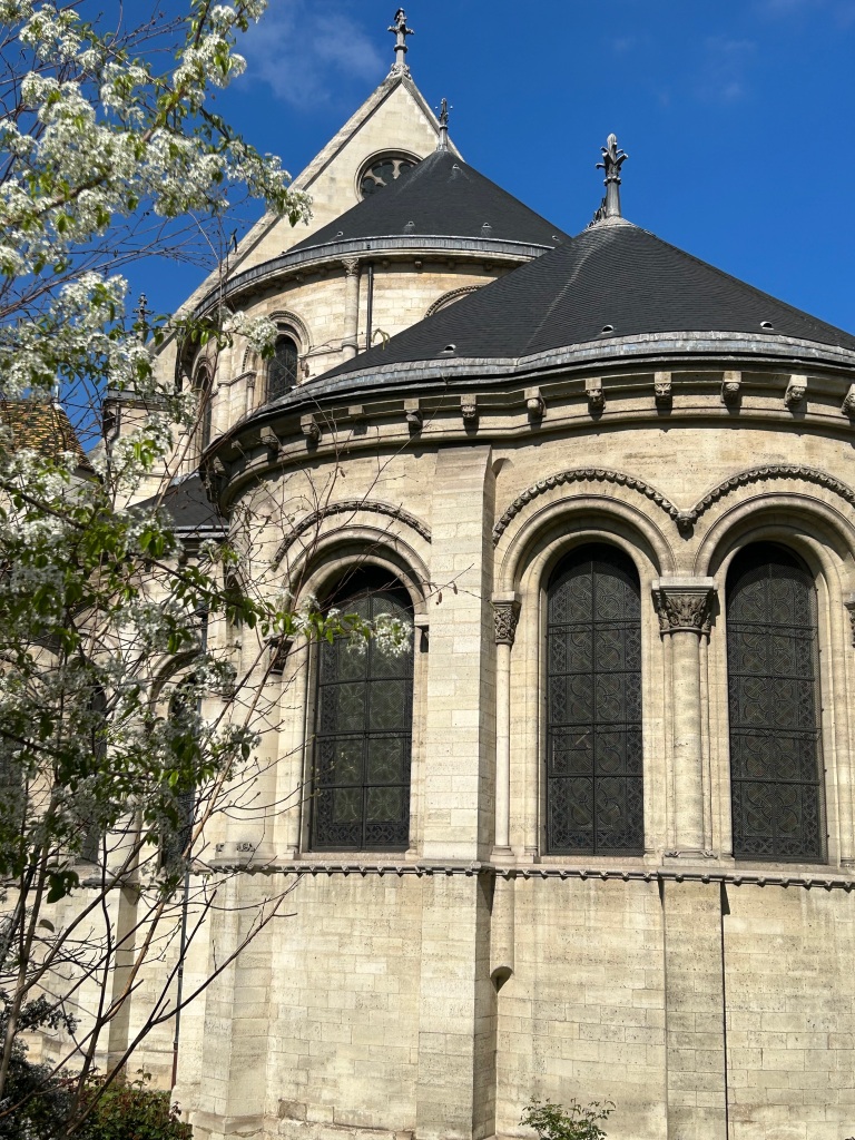
I made the pilgrimage this spring. I was attending a quantum-chaos workshop at the Institut Pascal, an interdisciplinary institute in a suburb of Paris. One quiet Saturday morning, I rode a train into the city center. The city houses a former priory—a gorgeous, 11th-century, white-stone affair of the sort for which I envy European cities. For over 200 years, the former priory has housed the Musée des Arts et Métiers, a museum of industry and technology. In the priory’s chapel hangs Foucault’s pendulum.2

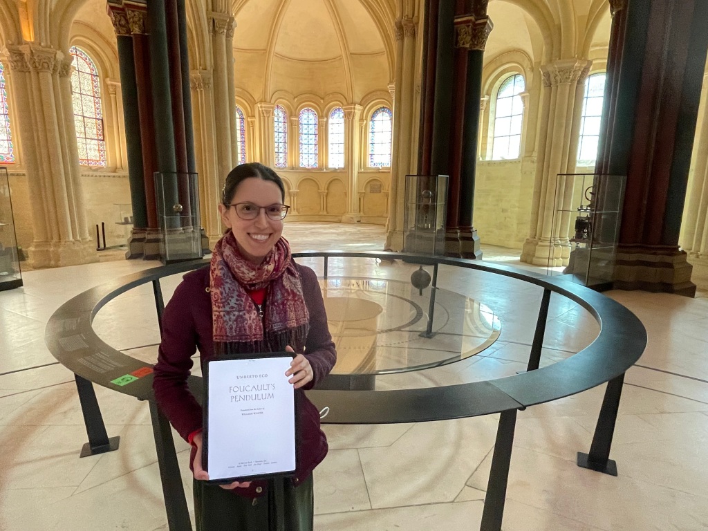
A pendulum of Foucault’s own—the one he exhibited at the Panthéon—used to hang in the chapel. That pendulum broke in 2010; but still, the pendulum swinging today is all but a holy relic of scientific history. Foucault’s pendulum! Demonstrating that the Earth rotates! And in a jewel of a setting—flooded with light from stained-glass windows and surrounded by Gothic arches below a painted ceiling. I flitted around the little chapel like a pollen-happy bee for maybe 15 minutes, watching the pendulum swing, looking at other artifacts of Foucault’s, wending my way around the carved columns.

Almost alone. A handful of visitors trickled in and out. They contrasted with my visit, the previous weekend, to the Louvre. There, I’d witnessed a Disney World–esque line of tourists waiting for a glimpse of the Mona Lisa, camera phones held high. Nobody was queueing up in the musée’s chapel. But this was Foucault’s pendulum! Demonstrating that the Earth rotates!

I confess to capitalizing on the lack of visitors to take a photo with Foucault’s pendulum and Foucault’s Pendulum, though.

Shortly before I’d left for Paris, a librarian friend had recommended Umberto Eco’s novel Foucault’s Pendulum. It occupied me during many a train ride to or from the center of Paris.

The rest of the museum could model in an advertisement for steampunk. I found automata, models of the steam engines that triggered the Industrial Revolution, and a phonograph of Thomas Edison’s. The gadgets, many formed from brass and dark wood, contrast with the priory’s light-toned majesty. Yet the priory shares its elegance with the inventions, many of which gleam and curve in decorative flutes. 

The grand finale at the Musée des Arts et Métiers.

I tore myself away from the Musée des Arts et Métiers after several hours. I returned home a week later and heard the song “Fireflies” again not long afterward. The goosebumps returned worse. Thanks to Foucault, I can make myself believe that planet Earth turns.

With thanks to Kristina Lynch for tolerating my many, many, many questions throughout her classical-mechanics course.

This story’s title refers to a translation of Goethe’s Faust. In the translation, the demon Mephistopheles tells the title character, “You let the great world spin and riot; / we’ll nest contented in our quiet” (to within punctuational and other minor errors, as I no longer have the text with me). A prize-winning 2009 novel is called Let the Great World Spin; I’ve long wondered whether Faust inspired its title.

1Why isn’t the bottom of the pendulum called the alice?

2After visiting the musée, I learned that my classical-mechanics professor had been referring to the Foucault pendulum that hangs in the Panthéon, rather than to the pendulum in the musée. The musée still contains the pendulum used by Foucault in 1851, whereas the Panthéon has only a copy, so I’m content. Still, I wouldn’t mind making a pilgrimage to the Panthéon. Let me know if more thermodynamic workshops take place in Paris!

Quantum computing vs. Grubhub

pon receiving my speaking assignments for the Tucson Festival of Books, I mentally raised my eyebrows. I’d be participating in a panel discussion with Mike Evans, the founder of Grubhub? But I hadn’t created an app that’s a household name. I hadn’t transformed 30 million people’s eating habits. I’m a theoretical physicist; I build universes in my head for a living. I could spend all day trying to prove a theorem and failing, and no stocks would tumble as a result.

Once the wave of incredulity had crested, I noticed that the panel was entitled “The Future of Tech.” Grubhub has transformed technology, I reasoned, and quantum computing is in the process of doing so. Fair enough. 

Besides, my husband pointed out, the food industry requires fridges. Physicists building quantum computers from superconductors need fridges. The latter fridges require temperatures ten million times lower than restaurateurs do, but we still share an interest.

Very well, I thought. Game on.

Tucson hosts the third-largest book festival in the United States. And why shouldn’t it, as the festival takes place in early March, when much of the country is shivering and eyeing Arizona’s T-shirt temperatures with envy? If I had to visit any institution in the winter, I couldn’t object to the festival’s home, the University of Arizona.

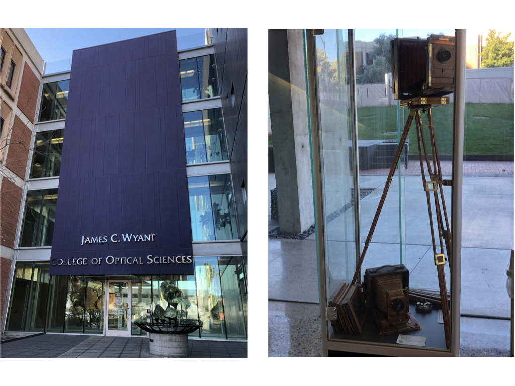
The day before the festival, I presented a colloquium at the university, for the Arizona Quantum Alliance. The talk took place in the Wyant College of Optical Sciences, the home of an optical-instruments museum. Many of the instruments date to the 1800s and, built from brass and wood, smack of steampunk. I approved. Outside the optics building, workers were setting up tents to house the festival’s science activities.

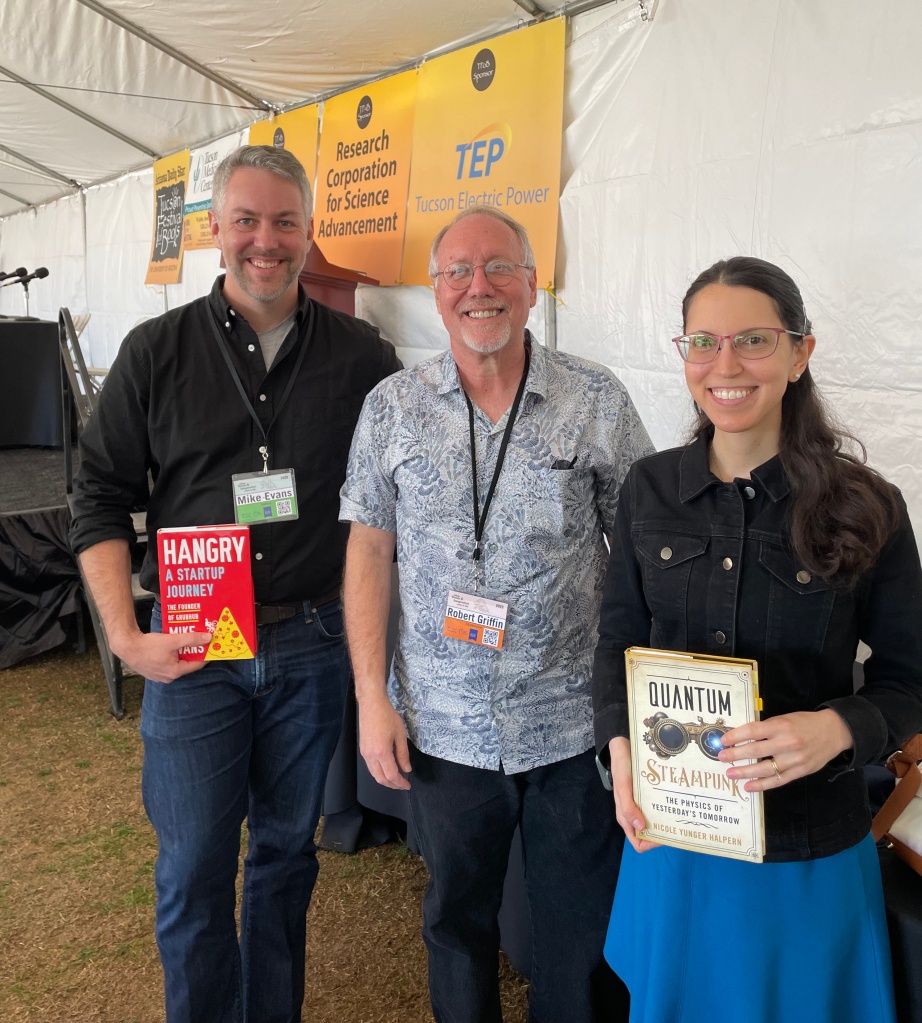
The next day—a Saturday—dawned clear and bright. Late in the morning, I met Mike and our panel’s moderator, Bob Griffin, another startup veteran. We sat down at a table in the back of a broad tent, the tent filled up with listeners, and the conversation began.

I relished the conversation as I’d relished an early-morning ramble along the trails by my hotel at the base of the Santa Catalina Mountains. I joined theoretical physics for the love of ideas, and this exchange of ideas offered an intellectual workout. One of Mike’s points resonated with me most: Grubhub didn’t advance technology much. He shifted consumers from ordering pizza via phone call to ordering pizza via computer, then to ordering pizza via apps on phones. Yet these small changes, accumulated across a population and encouraged by a pandemic, changed society. Food-delivery services exploded and helped establish the gig economy (despite Mike’s concerns about worker security). One small step for technology, adopted by tens of millions, can constitute one giant leap for commerce.

To me, Grubhub offered a foil for quantum computing, which offers a giant leap in technology: The physical laws best-suited to describing today’s computers can’t describe quantum computers. Some sources portray this advance as bound to transform all our lives in countless ways. This portrayal strikes some quantum scientists as hype that can endanger quality work. 

Quantum computers will transform cybersecurity, being able to break the safeguards that secure our credit-card information when we order food via Grubhub. Yet most consumers don’t know what safeguards are protecting us. We simply trust that safeguards exist. How they look under the hood will change by the time large-scale quantum computers exist—will metamorphose perhaps as dramatically as did Gregor Samsa before he woke up as an insect. But consumers’ lives might not metamorphose.

Quantum scientists hope and anticipate that quantum computers will enable discoveries in chemistry, materials science, and pharmacology. Molecules are quantum, and many materials exhibit quantum properties. Simulating quantum systems takes classical (everyday) computers copious amounts of time and memory—in some cases, so much that a classical computer the size of the universe would take ages. Quantum computers will be able to simulate quantum subjects naturally. But how these simulations will impact everyday life remains a question.

For example, consider my favorite potential application of quantum computers: fertilizer production, as envisioned by Microsoft’s quantum team. Humanity spends about 3% of the world’s energy on producing fertilizer, using a technique developed in 1909. Bacteria accomplish the same goal far more efficiently. But those bacteria use a molecule—nitrogenase—too complicated for us to understand using classical computers. Being quantum, the molecule invites quantum computation. Quantum computers may crack the molecule’s secrets and transform fertilizer production and energy use. The planet and humanity would benefit. We might reduce famines or avert human-driven natural disasters. But would the quantum computation change my neighbor’s behavior as Grubhub has? I can’t say.

Finally, evidence suggests that quantum computers can assist with optimization problems. Imagine a company that needs to transport supplies to various places at various times. How can the company optimize this process—implement it most efficiently? Quantum computers seem likely to be able to help. The evidence isn’t watertight, however, and quantum computers might not solve optimization problems exactly. If the evidence winds up correct, industries will benefit. But would this advance change Jane Doe’s everyday habits? Or will she only receive pizza deliveries a few minutes more quickly?

Don’t get me wrong; quantum technology has transformed our lives. It’s enabled the most accurate, most precise clocks in the world, which form the infrastructure behind GPS. Quantum physics has awed us, enabling the detection of gravitational waves—ripples, predicted by Einstein, in spacetime. But large-scale quantum computers—the holy grail of quantum technology—don’t suit all problems, such as totting up the miles I traveled en route to Tucson; and consumers might not notice quantum computers’ transformation of cybersecurity. I expect quantum computing to change the world, but let’s think twice about whether quantum computing will change everyone’s life like a blockbuster app.

I’ve no idea how many people have made this pun about Mike’s work, but the panel discussion left me with food for thought. He earned his undergraduate degree at MIT, by the way; so scientifically inclined Quantum Frontiers readers might enjoy his memoir, Hangry. It conveys a strong voice and dishes on data and diligence through stories. (For the best predictor of whether you’ll enjoy a burrito, ignore the starred reviews. Check how many people have reordered the burrito.)

The festival made my week. After the panel, I signed books; participated in a discussion about why “The Future Is Quantum!” with law professor Jane Bambauer; and narrowly missed a talk by Lois Lowry, a Newbury Award winner who wrote novels that I read as a child. (The auditorium filled up before I reached the door, but I’m glad that it did; Lois Lowry deserves a packed house and then some.) I learned—as I’d wondered—that yes, there’s something magical to being an author at a book festival. And I learned about how the future of tech depends on more than tech.

Memories of things past

My best friend—who’s held the title of best friend since kindergarten—calls me the keeper of her childhood memories. I recall which toys we played with, the first time I visited her house,1 and which beverages our classmates drank during snack time in kindergarten.2 She wouldn’t be surprised to learn that the first workshop I’ve co-organized centered on memory.

Memory—and the loss of memory—stars in thermodynamics. As an example, take what my husband will probably do this evening: bake tomorrow’s breakfast. I don’t know whether he’ll bake fruit-and-oat cookies, banana muffins, pear muffins, or pumpkin muffins. Whichever he chooses, his baking will create a scent. That scent will waft across the apartment, seep into air vents, and escape into the corridor—will disperse into the environment. By tomorrow evening, nobody will be able to tell by sniffing what my husband will have baked. 

That is, the kitchen’s environment lacks a memory. This lack contributes to our experience of time’s arrow: We sense that time passes partially by smelling less and less of breakfast. Physicists call memoryless systems and processes Markovian.

Our kitchen’s environment is Markovian because it’s large and particles churn through it randomly. But not all environments share these characteristics. Metaphorically speaking, a dispersed memory of breakfast may recollect, return to a kitchen, and influence the following week’s baking. For instance, imagine an atom in a quantum computer, rather than a kitchen in an apartment. A few other atoms may form our atom’s environment. Quantum information may leak from our atom into that environment, swish around in the environment for a time, and then return to haunt our atom. We’d call the atom’s evolution and environment non-Markovian.

I had the good fortune to co-organize a workshop about non-Markovianity—about memory—this February. The workshop took place at the Banff International Research Station, abbreviated BIRS, which you pronounce like the plural of what you say when shivering outdoors in Canada. BIRS operates in the Banff Centre for Arts and Creativity, high in the Rocky Mountains. The Banff Centre could accompany a dictionary entry for pristine, to my mind. The air feels crisp, the trees on nearby peaks stand out against the snow like evergreen fringes on white velvet, and the buildings balance a rustic-mountain-lodge style with the avant-garde. 

The workshop balanced styles, too, but skewed toward the theoretical and abstract. We learned about why the world behaves classically in our everyday experiences; about information-theoretic measures of the distances between quantum states; and how to simulate, on quantum computers, chemical systems that interact with environments. One talk, though, brought our theory back down to (the snow-dusted) Earth.

Gabriela Schlau-Cohen runs a chemistry lab at MIT. She wants to understand how plants transport energy. Energy arrives at a plant from the sun in the form of light. The light hits a pigment-and-protein complex. If the plant is lucky, the light transforms into a particle-like packet of energy called an exciton. The exciton traverses the receptor complex, then other complexes. Eventually, the exciton finds a spot where it can enable processes such as leaf growth. 

A high fraction of the impinging photons—85%—transform into excitons. How do plants convert and transport energy as efficiently as they do?

Gabriela’s group aims to find out—not by testing natural light-harvesting complexes, but by building complexes themselves. The experimentalists mimic the complex’s protein using DNA. You can fold DNA into almost any shape you want, by choosing the DNA’s base pairs (basic units) adroitly and by using “staples” formed from more DNA scraps. The sculpted molecules are called DNA origami.

Gabriela’s group engineers different DNA structures, analogous to complexes’ proteins, to have different properties. For instance, the experimentalists engineer rigid structures and flexible structures. Then, the group assesses how energy moves through each structure. Each structure forms an environment that influences excitons’ behaviors, similarly to how a memory-containing environment influences an atom.

Courtesy of Gabriela Schlau-Cohen

The Banff environment influenced me, stirring up memories like powder displaced by a skier on the slopes above us. I first participated in a BIRS workshop as a PhD student, and then I returned as a postdoc. Now, I was co-organizing a workshop to which I brought a PhD student of my own. Time flows, as we’re reminded while walking down the mountain from the Banff Centre into town: A cemetery borders part of the path. Time flows, but we belong to that thermodynamically remarkable class of systems that retain memories…memories and a few other treasures that resist change, such as friendships held since kindergarten.

1Plushy versions of Simba and Nala from The Lion King. I remain grateful to her for letting me play at being Nala.

2I’d request milk, another kid would request apple juice, and everyone else would request orange juice.