Discoveries at the Dibner

This past summer, our quantum thermodynamics research group had the wonderful opportunity to visit the Dibner Rare Book Library in D.C. Located in a small corner of the Smithsonian National Museum of American History, tucked away behind flashier exhibits, the Dibner is home to thousands of rare books and manuscripts, some dating back many centuries.

Our advisor, Nicole Yunger Halpern, has a special connection to the Dibner, having interned there as an undergrad. She’s remained in contact with the head librarian, Lilla Vekerdy. For our visit, the two of them curated a large spread of scientific work related to thermodynamics, physics, and mathematics. The tomes ranged from a 1500s print of Euclid’s Elements to originals of Einstein’s manuscripts with hand-written notes in the margin.

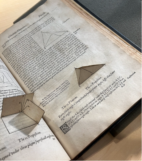
The print of Euclid’s Elements was one of the standout exhibits. It featured a number of foldout nets of 3D solids, which had been cut and glued into the book by hand. Several hundred copies of this print are believed to have been made, each of them containing painstakingly crafted paper models. At the time, this technique was an innovation, resulting from printers’ explorations of the then-young art of large-scale book publication.
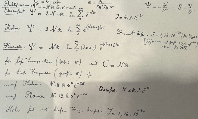
Another interesting exhibit was rough notes on ideal gases written by Planck, one of the fathers of quantum mechanics. Ideal gases are the prototypical model in statistical mechanics, capturing to high accuracy the behaviour of real gases within certain temperatures and pressures. The notes contained comparisons between BoltzmannEhrenfest, and Planck’s own calculations for classical and quantum ideal gases. Though the prose was in German, some results were instantly recognizable, such as the plot of the specific heat of a classical ideal gas, showing the stepwise jump as degrees of freedom freeze out. 
Looking through these great physicists’ rough notes, scratched-out ideas, and personal correspondences was a unique experience, helping humanize them and place their work in historical context. Understanding the history of science doesn’t just need to be for historians, it can be useful for scientists themselves! Seeing how scientists persevered through unknowns, grappling with doubts and incomplete knowledge to generate new ideas, is inspiring. But when one only reads the final, polished result in a modern textbook, it can be difficult to appreciate this process of discovery. Another reason to study the historical development of scientific results is that core concepts have a way of arising time and again across science. Recognizing how these ideas have arisen in the past is insightful. Examining the creative processes of great scientists before us helps develop our own intuition and skillset.

Thanks to our advisor for this field trip – and make sure to check out the Dibner next time you’re in DC! 

Good news everyone! Flatland is non-contextual!

Quantum mechanics is weird! Imagine for a second that you want to make an experiment and that the result of your experiment depends on what your colleague is doing in the next room. It would be crazy to live in such a world! This is the world we live in, at least at the quantum scale. The result of an experiment cannot be described in a way that is independent of the context. The neighbor is sticking his nose in our experiment!

Before telling you why quantum mechanics is contextual, let me give you an experiment that admits a simple non-contextual explanation. This story takes place in Flatland, a two-dimensional world inhabited by polygons. Our protagonist is a square who became famous after claiming that he met a sphere.

flatland


This square, call him Mr Square for convenience, met a sphere, Miss Sphere. When you live in a planar world like Flatland, this kind of event is not only rare, but it is also quite weird! For people of Flatland, only the intersection of Miss Sphere’s body with the plane is visible. Depending on the position of the sphere, its shape in Flatland will either be a point, a circle, or it could even be empty.

fut_egg

During their trip to flatland, Professor Farnsworth explains to Bender: “If we were in the third dimension looking down, we would be able to see an unhatched chick in it. Just as a chick in a 3-dimensional egg could be seen by an observer in the fourth dimension.’

Not convinced by Miss Sphere’s arguments, Mr Square tried to prove that she cannot exist – Square was a mathematician – and failed miserably. Let’s imagine a more realistic story, a story where spheres cannot speak. In this story, Mr Square will be a physicist, familiar with hidden variable models. Mr Square met a sphere, but a tongue-tied sphere! Confronted with this mysterious event, he did what any other citizen of Flatland would have done. He took a selfie with Miss Sphere. Mr Square was kind enough to let us use some of his photos to illustrate our story.

pics.png

Picture taken by Mr Square, with his Flatland-camera. (a) The sphere. (b) Selfie of Square (left) with the sphere (right).

As you can see on these photos, when you are stuck in Flatland and you take a picture of a sphere, only a segment is visible. What aroused Mr Square’s curiosity is the fact that the length of this segment changes constantly. Each picture shows a segment of a different length, due to the movement of the sphere along the z-axis, invisible to him. However, although they look random, Square discovered that these changing lengths can be explained without randomness by introducing a hidden variable living in a hypothetical third dimension. The apparent randomness is simply a consequence of his incomplete knowledge of the system: The position along the hidden variable axis z is inaccessible! Of course, this is only a model, this third dimension is purely theoretical, and no one from Flatland will ever visit it.

What about quantum mechanics?

Measurement outcomes are random as well in the quantum realm. Can we explain the randomness in quantum measurements by a hidden variable? Surprisingly, the answer is no! Von Neumann, one of the greatest scientists of the 20th century, was the first one to make this claim in 1932. His attempt to prove this result is known today as “Von Neumann’s silly mistake”. It was not until 1966 that Bell convinced the community that Von Neumann’s argument relies on a silly assumption.

Consider first a system of a single quantum bit, or qubit. A qubit is a 2-level system. It can be either in a ground state or in an excited state, but also in a quantum superposition |\psi\rangle = \alpha |g\rangle + \beta|e\rangle of these two states, where \alpha and \beta are complex numbers such that |\alpha|^2 + |\beta|^2 = 1. We can see this quantum state as a 2-dimensional vector (\alpha, \beta), where the ground state is |g\rangle=(1,0) and the excited state is |e\rangle=(0,1).

projection

The probability of an outcome depends on the projection of the quantum state onto the ground state and the excited state.

What can we measure about this qubit? First, imagine that we want to know if our quantum state is in the ground state or in the excited state. There is a quantum measurement that returns a random outcome, which is g with probability P(g) = |\alpha|^2 and e with probability P(e) = |\beta|^2.

Let us try to reinterpret this measurement in a different way. Inspired by Mr Square’s idea, we extend our description of the state |\psi\rangle of the system to include the outcome as an extra parameter. In this model, a state is a pair of the form (|\psi\rangle, \lambda) where \lambda is either e or g. Our quantum state can be seen as being in position (|\psi\rangle, g) with probability P(g) or in position (|\psi\rangle, e) with probability P(e). Measuring only reveals the value of the hidden variable \lambda. By introducing a hidden variable, we made this measurement deterministic. This proves that the randomness can be moved to the level of the description of the state, just as in Flatland. The weirdness of quantum mechanics goes away.

Contextuality of quantum mechanics

Let us try to extend our hidden variable model to all quantum measurements. We can associate a measurement with a particular kind of matrix A, called an observable. Measuring an observable returns randomly one of its eigenvalue. For instance, the Pauli matrices

Z =  \begin{pmatrix}  1 & 0\\  0 & -1\\  \end{pmatrix}  \quad \text{ and } \quad  X =  \begin{pmatrix}  0 & 1\\  1 & 0\\  \end{pmatrix},

as well as Y = iZX and the identity matrix I, are 1-qubit observables with eigenvalues (i.e. measurement outcomes) \pm 1. Now, take a system of 2 qubits. Since each of the 2 qubits can be either excited or not, our quantum state is a 4-dimensional vector

|\psi\rangle = \alpha |g_1\rangle \otimes |g_2\rangle  + \beta |g_1\rangle \otimes |e_2\rangle  + \gamma |e_1\rangle \otimes |g_2\rangle  + \delta |e_1\rangle \otimes |e_2\rangle.

Therein, the 4 vectors |x\rangle \otimes |y\rangle can be identified with the vectors of the canonical basis (1000), (0100), (0010) and (0001). We will consider the measurement of 2-qubit observables of the form A \otimes B defined by A \otimes B |x\rangle \otimes |y\rangle = A |x\rangle \otimes B |y\rangle. In other words, A acts on the first qubit and B acts on the second one. Later, we will look into the observables X \otimes I, Z \otimes I, I \otimes X, I \otimes Z and their products.

What happens when two observables are measured simultaneously? In quantum mechanics, we can measure simultaneously multiple observables if these observables commute with each other. In that case, measuring O then O', or measuring O' first and then O, doesn’t make any difference. Therefore, we say that these observables are measured simultaneously, the outcome being a pair (\lambda,\lambda'), composed of an eigenvalue of O and an eigenvalue of O'. Their product O'' = OO', which commutes with both O and O', can also be measured in the same time. Measuring this triple returns a triple of eigenvalues (\lambda,\lambda',\lambda'') corresponding respectively to O, O' and O''. The relation O'' = OO' imposes the constraint

(1)               \qquad \lambda'' = \lambda \lambda'

on the outcomes.

Assume that one can describe the result of all quantum measurements with a model such that, for all observables O and for all states \nu of the model, a deterministic outcome \lambda_\nu(O) exists. Here, \nu is our ‘extended’, not necessarily physical, description of the state of the system. When O and O' are commuting, it is reasonable to assume that the relation (1) holds also at the level of the hidden variable model, namely

(2)                \lambda_\nu(OO') = \lambda_\nu(O) \cdot \lambda_\nu(O').

Such a model is called a non-contextual hidden variable model. Von Neumann proved that no such value \lambda_\nu exists by considering these relations for all pairs O, O' of observables. This shows that quantum mechanics is contextual! Hum… Wait a minute. It seems silly to impose such a constraint for all pairs of observable, including those that cannot be measured simultaneously. This is “Von Neumann’s silly assumption’. Only pairs of commuting observables should be considered.

mermin

Peres-Mermin proof of contextuality

One can resurrect Von Neumann’s argument, assuming Eq.(2) only for commuting observables. Peres-Mermin’s square provides an elegant proof of this result. Form a 3 \times 3 array with these observables. It is constructed in such a way that

(i) The eigenvalues of all the observables in Peres-Mermin’s square are ±1,

(ii) Each row and each column is a triple of commuting observables,

(iii) The last element of each row and each column is the product of the 2 first observables, except in the last column where Y \otimes Y = -(Z \otimes Z)(X \otimes X).

If a non-contextual hidden variable exists, it associates fixed eigenvalues a, b, c, d (which are either 1 or -1) with the 4 observables X \otimes I, Z \otimes I, I \otimes X, I \otimes Z. Applying Eq.(2) to the first 2 rows and to the first 2 columns, one deduces the values of all the observables of the square, except Y \otimes Y . Finally, what value should be attributed to Y \otimes Y? By (iii), applying Eq.(2) to the last row, one gets \lambda_\nu(Y \otimes Y) = abcd. However, using the last column, (iii) and Eq.(2) yield the opposite value \lambda_\nu (Y \otimes Y ) = -abcd. This is the expected contradiction, proving that there is no non-contextual value \lambda_\nu. Quantum mechanics is contextual!

We saw that the randomness in quantum measurements cannot be explained in a ‘classical’ way. Besides its fundamental importance, this result also influences quantum technologies. What I really care about is how to construct a quantum computer, or more generally, I would like to understand what kind of quantum device could be superior to its classical counterpart for certain tasks. Such a quantum advantage can only be reached by exploiting the weirdness of quantum mechanics, such as contextuality 1,2,3,4,5. Understanding these weird phenomena is one of the first tasks to accomplish.