My experimental adventures in quantum thermodynamics

Imagine a billiard ball bouncing around on a pool table. High-school level physics enables us to predict its motion until the end of time using simple equations for energy and momentum conservation, as long as you know the initial conditions – how fast the ball is moving at launch, and in which direction.

What if you add a second ball? This makes things more complicated, but predicting the future state of this system would still be possible based on the same principles. What about if you had a thousand balls, or a million? Technically, you could still apply the same equations, but the problem would not be tractable in any practical sense.

Billiard balls bouncing around on a pool table are a good analogy for a many-body system like a gas of molecules. Image credit

Thermodynamics lets us make precise predictions about averaged (over all the particles) properties of complicated, many-body systems, like millions of billiard balls or atoms bouncing around, without needing to know the gory details. We can make these predictions by introducing the notion of probabilities. Even though the system is deterministic – we can in principle calculate the exact motion of every ball – there are so many balls in this system, that the properties of the whole will be very close to the average properties of the balls. If you throw a six-sided die, the result is in principle deterministic and predictable, based on the way you throw it, but it’s in practice completely random to you – it could be 1 through 6, equally likely. But you know that if you cast a thousand dice, the average will be close to 3.5 – the average of all possibilities. Statistical physics enables us to calculate a probability distribution over the energies of the balls, which tells us everything about the average properties of the system. And because of entropy – the tendency for the system to go from ordered to disordered configurations, even if the probability distribution of the initial system is far from the one statistical physics predicts, after the system is allowed to bounce around and settle, this final distribution will be extremely close to a generic distribution that depends on average properties only. We call this the thermal distribution, and the process of the system mixing and settling to one of the most likely configurations – thermalization.

For a practical example – instead of billiard balls, consider a gas of air molecules bouncing around. The average energy of this gas is proportional to its temperature, which we can calculate from the probability distribution of energies. Being able to predict the temperature of a gas is useful for practical things like weather forecasting, cooling your home efficiently, or building an engine. The important properties of the initial state we needed to know – energy and number of particles – are conserved during the evolution, and we call them “thermodynamic charges”. They don’t actually need to be electric charges, although it is a good example of something that’s conserved.

Let’s cross from the classical world – balls bouncing around – to the quantum one, which deals with elementary particles that can be entangled, or in a superposition. What changes when we introduce this complexity? Do systems even thermalize in the quantum world? Because of the above differences, we cannot in principle be sure that the mixing and settling of the system will happen just like in the classical cases of balls or gas molecules colliding.
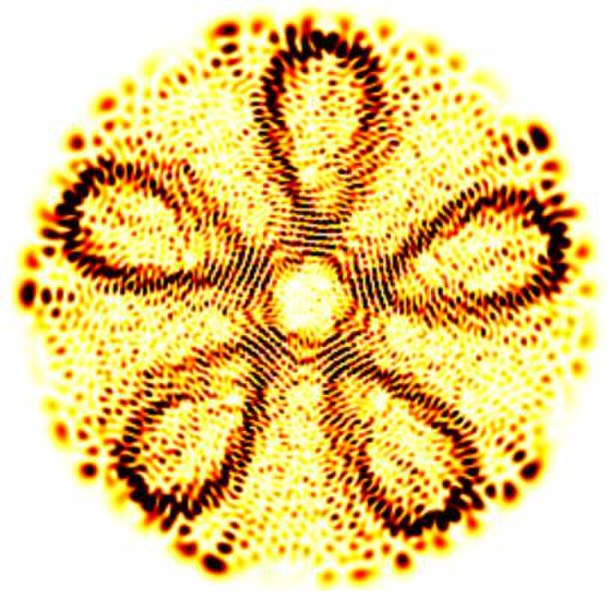
A visualization of a complex pattern called a quantum scar that can develop in quantum systems. Image credit

It turns out that we can predict the thermal state of a quantum system using very similar principles and equations that let us do this in the classical case. Well, with one exception – what if we cannot simultaneously measure our critical quantities – the charges?

One of the quirks of quantum mechanics is that observing the state of the system can change it. Before the observation, the system might be in a quantum superposition of many states. After the observation, a definite classical value will be recorded on our instrument – we say that the system has collapsed to this state, and thus changed its state. There are certain observables that are mutually incompatible – we cannot know their values simultaneously, because observing one definite value collapses the system to a state in which the other observable is in a superposition. We call these observables noncommuting, because the order of observation matters – unlike in multiplication of numbers, which is a commuting operation you’re familiar with. 2 * 3 = 6, and also 3 * 2 = 6 – the order of multiplication doesn’t matter.

Electron spin is a common example that entails noncommutation. In a simplified picture, we can think of spin as an axis of rotation of our electron in 3D space. Note that the electron doesn’t actually rotate in space, but it is a useful analogy – the property is “spin” for a reason. We can measure the spin along the x-,y-, or z-axis of a 3D coordinate system and obtain a definite positive or negative value, but this observation will result in a complete loss of information about spin in the other two perpendicular directions.
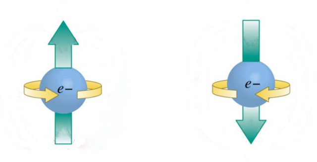
An illustration of electron spin. We can imagine it as an axis in 3D space that points in a particular direction. Image from Wikimedia Commons.

If we investigate a system that conserves the three spin components independently, we will be in a situation where the three conserved charges do not commute. We call them “non-Abelian” charges, because they enjoy a non-Abelian, that is, noncommuting, algebra. Will such a system thermalize, and if so, to what kind of final state?

This is precisely what we set out to investigate. Noncommutation of charges breaks usual derivations of the thermal state, but researchers have managed to show that with non-Abelian charges, a subtly different non-Abelian thermal state (NATS) should emerge. Myself and Nicole Yunger Halpern at the Joint Center for Quantum Information and Computer Science (QuICS) at the University of Maryland have collaborated with Amir Kalev from the Information Sciences Institute (ISI) at the University of Southern California, and experimentalists from the University of Innsbruck (Florian Kranzl, Manoj Joshi, Rainer Blatt and Christian Roos) to observe thermalization in a non-Abelian system – and we’ve recently published this work in PRX Quantum .

The experimentalists used a device that can trap ions with electric fields, as well as manipulate and read out their states using lasers. Only select energy levels of these ions are used, which effectively makes them behave like electrons. The laser field can couple the ions in a way that approximates the Heisenberg Hamiltonian – an interaction that conserves the three total spin components individually. We thus construct the quantum system we want to study – multiple particles coupled with interactions that conserve noncommuting charges.

We conceptually divide the ions into a system of interest and an environment. The system of interest, which consists of two particles, is what we want to measure and compare to theoretical predictions. Meanwhile, the other ions act as the effective environment for our pair of ions – the environment ions interact with the pair in a way that simulates a large bath exchanging heat and spin.
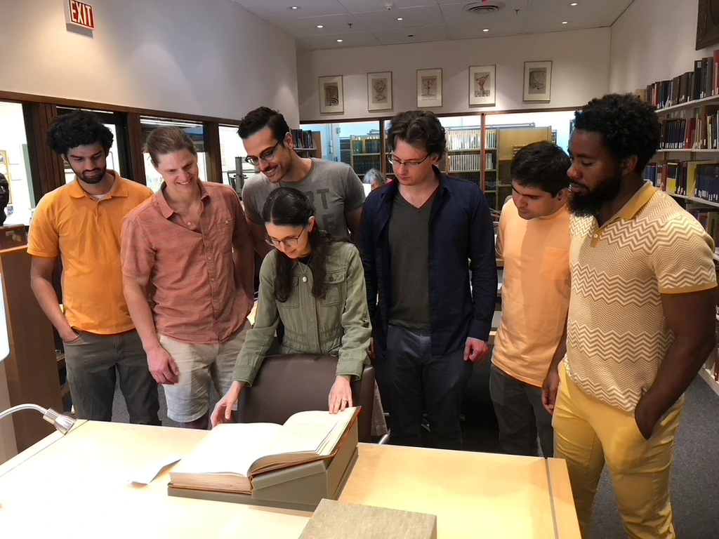
Photo of our University of Maryland group. From left to right: Twesh Upadhyaya, Billy Braasch, Shayan Majidy, Nicole Yunger Halpern, Aleks Lasek, Jose Antonio Guzman, Anthony Munson.

If we start this total system in some initial state, and let it evolve under our engineered interaction for a long enough time, we can then measure the final state of the system of interest. To make the NATS distinguishable from the usual thermal state, I designed an initial state that is easy to prepare, and has the ions pointing in directions that result in high charge averages and relatively low temperature. High charge averages make the noncommuting nature of the charges more pronounced, and low temperature makes the state easy to distinguish from the thermal background. However, we also show that our experiment works for a variety of more-arbitrary states.

We let the system evolve from this initial state for as long as possible given experimental limitations, which was 15 ms. The experimentalists then used quantum state tomography to reconstruct the state of the system of interest. Quantum state tomography makes multiple measurements over many experimental runs to approximate the average quantum state of the system measured. We then check how close the measured state is to the NATS. We have found that it’s about as close as one can expect in this experiment!

And we know this because we have also implemented a different coupling scheme, one that doesn’t have non-Abelian charges. The expected thermal state in the latter case was reached within a distance that’s a little smaller than our non-Abelian case. This tells us that the NATS is almost reached in our experiment, and so it is a good, and the best known, thermal state for the non-Abelian system – we have compared it to competitor thermal states.

Working with the experimentalists directly has been a new experience for me. While I was focused on the theory and analyzing the tomography results they obtained, they needed to figure out practical ways to realize what we asked of them. I feel like each group has learned a lot about the tasks of the other. I have become well acquainted with the trapped ion experiment and its capabilities and limitation. Overall, it has been great collaborating with the Austrian group.

Our result is exciting, as it’s the first experimental observation within the field of non-Abelian thermodynamics! This result was observed in a realistic, non-fine-tuned system that experiences non-negligible errors due to noise. So the system does thermalize after all. We have also demonstrated that the trapped ion experiment of our Austrian friends can be used to simulate interesting many-body quantum systems. With different settings and programming, other types of couplings can be simulated in different types of experiments.

The experiment also opened avenues for future work. The distance to the NATS was greater than the analogous distance to the Abelian system. This suggests that thermalization is inhibited by the noncommutation of charges, but more evidence is needed to justify this claim. In fact, our other recent paper in Physical Review B suggests the opposite!

As noncommutation is one of the core features that distinguishes classical and quantum physics, it is of great interest to unravel the fine differences non-Abelian charges can cause. But we also hope that this research can have practical uses. If thermalization is disrupted by noncommutation of charges, engineered systems featuring them could possibly be used to build quantum memory that is more robust, or maybe even reduce noise in quantum computers. We continue to explore noncommutation, looking for interesting effects that we can pin on it. I am currently working on verifying the workings of a hypothesis that explains when and why quantum systems thermalize internally.

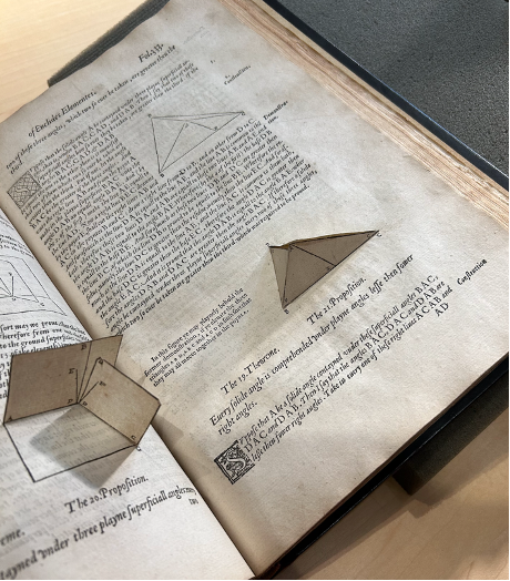
Discoveries at the Dibner

This past summer, our quantum thermodynamics research group had the wonderful opportunity to visit the Dibner Rare Book Library in D.C. Located in a small corner of the Smithsonian National Museum of American History, tucked away behind flashier exhibits, the Dibner is home to thousands of rare books and manuscripts, some dating back many centuries.

Our advisor, Nicole Yunger Halpern, has a special connection to the Dibner, having interned there as an undergrad. She’s remained in contact with the head librarian, Lilla Vekerdy. For our visit, the two of them curated a large spread of scientific work related to thermodynamics, physics, and mathematics. The tomes ranged from a 1500s print of Euclid’s Elements to originals of Einstein’s manuscripts with hand-written notes in the margin.

The print of Euclid’s Elements was one of the standout exhibits. It featured a number of foldout nets of 3D solids, which had been cut and glued into the book by hand. Several hundred copies of this print are believed to have been made, each of them containing painstakingly crafted paper models. At the time, this technique was an innovation, resulting from printers’ explorations of the then-young art of large-scale book publication.

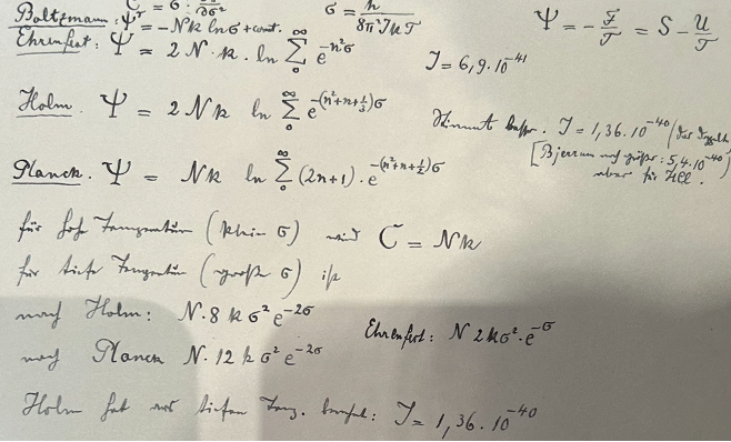
Another interesting exhibit was rough notes on ideal gases written by Planck, one of the fathers of quantum mechanics. Ideal gases are the prototypical model in statistical mechanics, capturing to high accuracy the behaviour of real gases within certain temperatures and pressures. The notes contained comparisons between BoltzmannEhrenfest, and Planck’s own calculations for classical and quantum ideal gases. Though the prose was in German, some results were instantly recognizable, such as the plot of the specific heat of a classical ideal gas, showing the stepwise jump as degrees of freedom freeze out. 

Looking through these great physicists’ rough notes, scratched-out ideas, and personal correspondences was a unique experience, helping humanize them and place their work in historical context. Understanding the history of science doesn’t just need to be for historians, it can be useful for scientists themselves! Seeing how scientists persevered through unknowns, grappling with doubts and incomplete knowledge to generate new ideas, is inspiring. But when one only reads the final, polished result in a modern textbook, it can be difficult to appreciate this process of discovery. Another reason to study the historical development of scientific results is that core concepts have a way of arising time and again across science. Recognizing how these ideas have arisen in the past is insightful. Examining the creative processes of great scientists before us helps develop our own intuition and skillset.

Thanks to our advisor for this field trip – and make sure to check out the Dibner next time you’re in DC! 

Good news everyone! Flatland is non-contextual!

Quantum mechanics is weird! Imagine for a second that you want to make an experiment and that the result of your experiment depends on what your colleague is doing in the next room. It would be crazy to live in such a world! This is the world we live in, at least at the quantum scale. The result of an experiment cannot be described in a way that is independent of the context. The neighbor is sticking his nose in our experiment!

Before telling you why quantum mechanics is contextual, let me give you an experiment that admits a simple non-contextual explanation. This story takes place in Flatland, a two-dimensional world inhabited by polygons. Our protagonist is a square who became famous after claiming that he met a sphere.

flatland


This square, call him Mr Square for convenience, met a sphere, Miss Sphere. When you live in a planar world like Flatland, this kind of event is not only rare, but it is also quite weird! For people of Flatland, only the intersection of Miss Sphere’s body with the plane is visible. Depending on the position of the sphere, its shape in Flatland will either be a point, a circle, or it could even be empty.

fut_egg

During their trip to flatland, Professor Farnsworth explains to Bender: “If we were in the third dimension looking down, we would be able to see an unhatched chick in it. Just as a chick in a 3-dimensional egg could be seen by an observer in the fourth dimension.’

Not convinced by Miss Sphere’s arguments, Mr Square tried to prove that she cannot exist – Square was a mathematician – and failed miserably. Let’s imagine a more realistic story, a story where spheres cannot speak. In this story, Mr Square will be a physicist, familiar with hidden variable models. Mr Square met a sphere, but a tongue-tied sphere! Confronted with this mysterious event, he did what any other citizen of Flatland would have done. He took a selfie with Miss Sphere. Mr Square was kind enough to let us use some of his photos to illustrate our story.

pics.png

Picture taken by Mr Square, with his Flatland-camera. (a) The sphere. (b) Selfie of Square (left) with the sphere (right).

As you can see on these photos, when you are stuck in Flatland and you take a picture of a sphere, only a segment is visible. What aroused Mr Square’s curiosity is the fact that the length of this segment changes constantly. Each picture shows a segment of a different length, due to the movement of the sphere along the z-axis, invisible to him. However, although they look random, Square discovered that these changing lengths can be explained without randomness by introducing a hidden variable living in a hypothetical third dimension. The apparent randomness is simply a consequence of his incomplete knowledge of the system: The position along the hidden variable axis z is inaccessible! Of course, this is only a model, this third dimension is purely theoretical, and no one from Flatland will ever visit it.

What about quantum mechanics?

Measurement outcomes are random as well in the quantum realm. Can we explain the randomness in quantum measurements by a hidden variable? Surprisingly, the answer is no! Von Neumann, one of the greatest scientists of the 20th century, was the first one to make this claim in 1932. His attempt to prove this result is known today as “Von Neumann’s silly mistake”. It was not until 1966 that Bell convinced the community that Von Neumann’s argument relies on a silly assumption.

Consider first a system of a single quantum bit, or qubit. A qubit is a 2-level system. It can be either in a ground state or in an excited state, but also in a quantum superposition |\psi\rangle = \alpha |g\rangle + \beta|e\rangle of these two states, where \alpha and \beta are complex numbers such that |\alpha|^2 + |\beta|^2 = 1. We can see this quantum state as a 2-dimensional vector (\alpha, \beta), where the ground state is |g\rangle=(1,0) and the excited state is |e\rangle=(0,1).

projection

The probability of an outcome depends on the projection of the quantum state onto the ground state and the excited state.

What can we measure about this qubit? First, imagine that we want to know if our quantum state is in the ground state or in the excited state. There is a quantum measurement that returns a random outcome, which is g with probability P(g) = |\alpha|^2 and e with probability P(e) = |\beta|^2.

Let us try to reinterpret this measurement in a different way. Inspired by Mr Square’s idea, we extend our description of the state |\psi\rangle of the system to include the outcome as an extra parameter. In this model, a state is a pair of the form (|\psi\rangle, \lambda) where \lambda is either e or g. Our quantum state can be seen as being in position (|\psi\rangle, g) with probability P(g) or in position (|\psi\rangle, e) with probability P(e). Measuring only reveals the value of the hidden variable \lambda. By introducing a hidden variable, we made this measurement deterministic. This proves that the randomness can be moved to the level of the description of the state, just as in Flatland. The weirdness of quantum mechanics goes away.

Contextuality of quantum mechanics

Let us try to extend our hidden variable model to all quantum measurements. We can associate a measurement with a particular kind of matrix A, called an observable. Measuring an observable returns randomly one of its eigenvalue. For instance, the Pauli matrices

Z =  \begin{pmatrix}  1 & 0\\  0 & -1\\  \end{pmatrix}  \quad \text{ and } \quad  X =  \begin{pmatrix}  0 & 1\\  1 & 0\\  \end{pmatrix},

as well as Y = iZX and the identity matrix I, are 1-qubit observables with eigenvalues (i.e. measurement outcomes) \pm 1. Now, take a system of 2 qubits. Since each of the 2 qubits can be either excited or not, our quantum state is a 4-dimensional vector

|\psi\rangle = \alpha |g_1\rangle \otimes |g_2\rangle  + \beta |g_1\rangle \otimes |e_2\rangle  + \gamma |e_1\rangle \otimes |g_2\rangle  + \delta |e_1\rangle \otimes |e_2\rangle.

Therein, the 4 vectors |x\rangle \otimes |y\rangle can be identified with the vectors of the canonical basis (1000), (0100), (0010) and (0001). We will consider the measurement of 2-qubit observables of the form A \otimes B defined by A \otimes B |x\rangle \otimes |y\rangle = A |x\rangle \otimes B |y\rangle. In other words, A acts on the first qubit and B acts on the second one. Later, we will look into the observables X \otimes I, Z \otimes I, I \otimes X, I \otimes Z and their products.

What happens when two observables are measured simultaneously? In quantum mechanics, we can measure simultaneously multiple observables if these observables commute with each other. In that case, measuring O then O', or measuring O' first and then O, doesn’t make any difference. Therefore, we say that these observables are measured simultaneously, the outcome being a pair (\lambda,\lambda'), composed of an eigenvalue of O and an eigenvalue of O'. Their product O'' = OO', which commutes with both O and O', can also be measured in the same time. Measuring this triple returns a triple of eigenvalues (\lambda,\lambda',\lambda'') corresponding respectively to O, O' and O''. The relation O'' = OO' imposes the constraint

(1)               \qquad \lambda'' = \lambda \lambda'

on the outcomes.

Assume that one can describe the result of all quantum measurements with a model such that, for all observables O and for all states \nu of the model, a deterministic outcome \lambda_\nu(O) exists. Here, \nu is our ‘extended’, not necessarily physical, description of the state of the system. When O and O' are commuting, it is reasonable to assume that the relation (1) holds also at the level of the hidden variable model, namely

(2)                \lambda_\nu(OO') = \lambda_\nu(O) \cdot \lambda_\nu(O').

Such a model is called a non-contextual hidden variable model. Von Neumann proved that no such value \lambda_\nu exists by considering these relations for all pairs O, O' of observables. This shows that quantum mechanics is contextual! Hum… Wait a minute. It seems silly to impose such a constraint for all pairs of observable, including those that cannot be measured simultaneously. This is “Von Neumann’s silly assumption’. Only pairs of commuting observables should be considered.

mermin

Peres-Mermin proof of contextuality

One can resurrect Von Neumann’s argument, assuming Eq.(2) only for commuting observables. Peres-Mermin’s square provides an elegant proof of this result. Form a 3 \times 3 array with these observables. It is constructed in such a way that

(i) The eigenvalues of all the observables in Peres-Mermin’s square are ±1,

(ii) Each row and each column is a triple of commuting observables,

(iii) The last element of each row and each column is the product of the 2 first observables, except in the last column where Y \otimes Y = -(Z \otimes Z)(X \otimes X).

If a non-contextual hidden variable exists, it associates fixed eigenvalues a, b, c, d (which are either 1 or -1) with the 4 observables X \otimes I, Z \otimes I, I \otimes X, I \otimes Z. Applying Eq.(2) to the first 2 rows and to the first 2 columns, one deduces the values of all the observables of the square, except Y \otimes Y . Finally, what value should be attributed to Y \otimes Y? By (iii), applying Eq.(2) to the last row, one gets \lambda_\nu(Y \otimes Y) = abcd. However, using the last column, (iii) and Eq.(2) yield the opposite value \lambda_\nu (Y \otimes Y ) = -abcd. This is the expected contradiction, proving that there is no non-contextual value \lambda_\nu. Quantum mechanics is contextual!

We saw that the randomness in quantum measurements cannot be explained in a ‘classical’ way. Besides its fundamental importance, this result also influences quantum technologies. What I really care about is how to construct a quantum computer, or more generally, I would like to understand what kind of quantum device could be superior to its classical counterpart for certain tasks. Such a quantum advantage can only be reached by exploiting the weirdness of quantum mechanics, such as contextuality 1,2,3,4,5. Understanding these weird phenomena is one of the first tasks to accomplish.

Making predictions in the multiverse

Image

I am a theoretical physicist at University of California, Berkeley. Last month, I attended a very interesting conference organized by Foundamental Questions Institute (FQXi) in Puerto Rico, and presented a talk about making predictions in cosmology, especially in the eternally inflating multiverse. I very much enjoyed discussions with people at the conference, where I was invited to post a non-technical account of the issue as well as my own view of it. So here I am.

I find it quite remarkable that some of us in the physics community are thinking with some “confidence” that we live in the multiverse, more specifically one of the many universes in which low-energy physical laws take different forms. (For example, these universes have different elementary particles with different properties, possibly different spacetime dimensions, and so on.) This idea of the multiverse, as we currently think, is not simply a result of random imagination by theorists, but is based on several pieces of observational and theoretical evidence.

Observationally, we have learned more and more that we live in a highly special universe—it seems that the “physical laws” of our universe (summarized in the form of standard models of particle physics and cosmology) takes such a special form that if its structure were varied slightly, then there would be no interesting structure in the universe, let alone intelligent life. It is hard to understand this fact unless there are many universes with varying “physical laws,” and we simply happen to emerge in a universe which allows for intelligent life to develop (which seems to require special conditions). With multiple universes, we can understand the “specialness” of our universe precisely as we understand the “specialness” of our planet Earth (e.g. the ideal distance from the sun), which is only one of the many planets out there.

Perhaps more nontrivial is the fact that our current theory of fundamental physics leads to this picture of the multiverse in a very natural way. Imagine that at some point in the history of the universe, space is exponentially expanding. This expansion—called inflation—occurs when space is filled with a “positive vacuum energy” (which happens quite generally). We knew, already in 80’s, that such inflation is generically eternal. During inflation, various non-inflating regions called bubble universes—of which our own universe could be one—may form, much like bubbles in boiling water. Since ambient space expands exponentially, however, these bubbles do not percolate; rather, the process of creating bubble universes lasts forever in an eternally inflating background. Now, recent progress in string theory suggests that low energy theories describing phyics in these bubble universes (such as the elementary particle content and their properties) may differ bubble by bubble. This is precisely the setup needed to understand the “specialness” of our universe because of the selection effect associated with our own existence, as described above.

multiverse

A schematic depiction of the eternally inflating multiverse. The horizontal and vertical directions correspond to spatial and time directions, respectively, and various regions with the inverted triangle or argyle shape represent different universes. While regions closer to the upper edge of the diagram look smaller, it is an artifact of the rescaling made to fit the large spacetime into a finite drawing—the fractal structure near the upper edge actually corresponds to an infinite number of large universes.

This particular version of the multiverse—called the eternally inflating multiverse—is very attractive. It is theoretically motivated and has a potential to explain various features seen in our universe. The eternal nature of inflation, however, causes a serious issue of predictivity. Because the process of creating bubble universes occurs infinitely many times, “In an eternally inflating universe, anything that can happen will happen; in fact, it will happen an infinite number of times,” as phrased in an article by Alan Guth. Suppose we want to calculate the relative probability for (any) events A and B to happen in the multiverse. Following the standard notion of probability, we might define it as the ratio of the numbers of times events A and B happen throughout the whole spacetime

P = \frac{N_A}{N_B}.

In the eternally inflating multiverse, however, both A and B occur infinitely many times: N_A, N_B = \infty. This expression, therefore, is ill-defined. One might think that this is merely a technical problem—we simply need to “regularize” to make both N_{A,B} finite, at a middle stage of the calculation, and then we get a well-defined answer. This is, however, not the case. One finds that depending on the details of this regularization procedure, one can obtain any “prediction” one wants, and there is no a priori preferred way to proceed over others—predictivity of physical theory seems lost!

Over the past decades, some physicists and cosmologists have been thinking about many aspects of this so-called measure problem in eternal inflation. (There are indeed many aspects to the problem, and I’m omitting most of them in my simplified presentation above.) Many of the people who contributed were in the session at the conference, including Aguirre, Albrecht, Bousso, Carroll, Guth, Page, Tegmark, and Vilenkin. My own view, which I think is shared by some others, is that this problem offers a window into deep issues associated with spacetime and gravity. In my 2011 paper I suggested that quantum mechanics plays a crucial role in understanding the multiverse, even at the largest distance scales. (A similar idea was also discussed here around the same time.) In particular, I argued that the eternally inflating multiverse and quantum mechanical many worlds a la Everett are the same concept:

Multiverse = Quantum Many Worlds

in a specific, and literal, sense. In this picture, the global spacetime of general relativity appears only as a derived concept at the cost of overcounting true degrees of freedom; in particular, infinitely large space associated with eternal inflation is a sort of “illusion.” A “true” description of the multiverse must be “intrinsically” probabilistic in a quantum mechanical sense—probabilities in cosmology and quantum measurements have the same origin.

To illustrate the basic idea, let us first consider an (apparently unrelated) system with a black hole. Suppose we drop some book A into the black hole and observe subsequent evolution of the system from a distance. The book will be absorbed into (the horizon of) the black hole, which will then eventually evaporate, leaving Hawking radiation. Now, let us consider another process of dropping a different book B, instead of A, and see what happens. The subsequent evolution in this case is similar to the case with A, and we will be left with Hawking radiation. However, this final-state Hawking radiation arising from B is (believed by many to be) different from that arising from A in its subtle quantum correlation structure, so that if we have perfect knowledge about the final-state radiation then we can reconstruct what the original book was. This property is called unitarity and is considered to provide the correct picture for black hole dynamics, based on recent theoretical progress. To recap, the information about the original book will not be lost—it will simply be distributed in final-state Hawking radiation in a highly scrambled form.

A puzzling thing occurs, however, if we observe the same phenomenon from the viewpoint of an observer who is falling into the black hole with a book. In this case, the equivalence principle says that the book does not feel gravity (except for the tidal force which is tiny for a large black hole), so it simply passes through the black hole horizon without any disruption. (Recently, this picture was challenged by the so-called firewall argument—the book might hit a collection of higher energy quanta called a firewall, rather than freely fall. Even if so, it does not affect our basic argument below.) This implies that all the information about the book (in fact, the book itself) will be inside the horizon at late times. On the other hand, we have just argued that from a distant observer’s point of view, the information will be outside—first on the horizon and then in Hawking radiation. Which is correct?

One might think that the information is simply duplicated: one copy inside and the other outside. This, however, cannot be the case. Quantum mechanics prohibits faithful copying of full quantum information, the so-called no-cloning theorem. Therefore, it seems that the two pictures by the two observers cannot both be correct.

The proposed solution to this puzzle is interesting—both pictures are correct, but not at the same time. The point is that one cannot be both a distant observer and a falling observer at the same time. If you are a distant observer, the information will be outside, and the interior spacetime must be viewed as non-existent since you can never access it even in principle (because of the existence of the horizon). On the other hand, if you are a falling observer, then you have the interior spacetime in which the information (the book itself) will fall, but this happens only at the cost of losing a part of spacetime in which Hawking radiation lies, which you can never access since you yourself are falling into the black hole. There is no inconsistency in either of these two pictures; only if you artificially “patch” the two pictures, which you cannot physically do, does the apparent inconsistency of information duplication occurs. This somewhat surprising aspect of a system with gravity is called black hole complementarity, pioneered by ‘t Hooft, Susskind, and their collaborators.

What does this discussion of black holes have to do with cosmology, and, in particular the eternally inflating multiverse? In cosmology our space is surrounded by a cosmological horizon. (For example, imagine that space is expanding exponentially; this makes it impossible for us to obtain any signal from regions farther than some distance because objects in these regions recede faster than speed of light. The definition of appropriate horizons in general cases is more subtle, but can be made.) The situation, therefore, is the “inside out” version of the black hole case viewed from a distant observer. As in the case of the black hole, quantum mechanics requires that spacetime on the other side of the horizon—in this case the exterior to the cosmological horizon—must be viewed as non-existent. (In the paper I made this claim based on some simple supportive calculations.) In a more technical term, a quantum state describing the system represents only the region within the horizon—there is no infinite space in any single, consistent description of the system!

If a quantum state represents only space within the horizon, then where is the multiverse, which we thought exists in an eternally inflating space further away from our own horizon? The answer is—probability! The process of creating bubble universes is a probabilistic process in the quantum mechanical sense—it occurs through quantum mechanical tunneling. This implies that, starting from some initially inflating space, we could end up with different universes probabilistically. All different universes—including our own—live in probability space. In a more technical term, a state representing eternally inflating space evolves into a superposition of terms—or branches—representing different universes, but with each of them representing only the region within its own horizon. Note that there is no concept of infinitely large space here, which led to the ill-definedness of probability. The picture of initially large multiverse, naively suggested by general relativity, appears only after “patching” pictures based on different branches together; but this vastly overcounts true degrees of freedom as was the case if we include both the interior spacetime and Hawking radiation in our description of a black hole.

The description of the multiverse presented here provides complete unification of the eternally inflating multiverse and the many worlds interpretation in quantum mechanics. Suppose the multiverse starts from some initial state |\Psi(t_0)\rangle. This state evolves into a superposition of states in which various bubble universes nucleate in various locations. As time passes, a state representing each universe further evolves into a superposition of states representing various possible cosmic histories, including different outcomes of “experiments” performed within that universe. (These “experiments” may, but need not, be scientific experiments—they can be any physical processes.) At late times, the multiverse state |\Psi(t)\rangle will thus contain an enormous number of terms, each of which represents a possible world that may arise from |\Psi(t_0)\rangle consistently with the laws of physics. Probabilities in cosmology and microscopic processes are then both given by quantum mechanical probabilities in the same manner. The multiverse and quantum many worlds are really the same thing—they simply refer to the same phenomenon occurring at (vastly) different scales.

branching

A schematic picture for the evolution of the multiverse state. As t increases, the state evolves into a superposition of states in which various bubble universes nucleate in various locations. Each of these states then evolves further into a superposition of states representing various possible cosmic histories, including different outcomes of experiments performed within that universe.

The picture presented here does not solve all the problems in eternally inflating cosmology. What is the actual quantum state of the multiverse? What is its “initial conditions”? What is time? How does it emerge? The picture, however, does provide a framework to address these further, deep questions, and I have recently made some progress: the basic idea is that the state of the multiverse (which may be selected uniquely by the normalizability condition) never changes, and yet time appears as an emergent concept locally in branches as physical correlations among objects (along the lines of an old idea by DeWitt). Given the length already, I will not elaborate on this new development here. If you are interested, you might want to read my paper.

It is fascinating that physicists can talk about big and deep questions like the ones discussed here based on concrete theoretical progress. Nobody really knows where these explorations will finally lead us to. It seems, however, clear that we live in an exciting era in which our scientific explorations reach beyond what we thought to be the entire physical world, our universe.

“Nature, you instruct me.”

“Settle thy studies.”

Alone in his workroom, a student contemplates his future. Piles of books teeter next to him. Boxes line the walls; and glass vials, the boxes. Sunbeams that struggle through the stained-glass window illuminate dust.

The student’s name is Faust. I met him during my last winter in college, while complementing Physics 42: Introductory Quantum Mechanics with German 44: The Faust Tradition. A medieval German alchemist, Faust has inspired plays, novels, operas, the short story “The Devil and Daniel Webster” about an American Congressman, and the film “Bedazzled” starring Brendan Frasier.

Image

The Faust tradition in popular culture. Mephistopheles is the demon who buys Faust’s soul. (http://xkcd.com/501/)

As I wondered what to pursue a PhD in, so (roughly speaking) did Faust. In plays by Christopher Marlowe and Johann Wolfgang von Goethe, Faust wavers among law, theology, philosophy, and medicine. You’ve probably heard what happens next: Faust chooses sorcery, conjures a demon, and bargains away his soul. Hardly the role model for a college student. I preferred to keep my soul, though Maxwell’s demon had stolen my heart.

A few decades after Goethe penned Faust, English physicist James Maxwell proposed a thought experiment. Consider a box divided into two rooms, he wrote, and a demon controlling the door between the rooms. Since others have explained Maxwell’s paradox, I won’t parrot them. Suffice to say, the demon helps clarify why time flows, what knowledge is, and how information relates to matter. Quantum-information physicists, I learned in a seminar after German 44, study Maxwell’s demon. Via the demon, experiment, and math, QI physicists study the whole world. I wanted to contemplate the whole world, like Goethe’s Faust. By studying QI, I might approximate my goal. Faust, almost as much as my QI seminar, convinced me to pursue a PhD in physics.

Fast forward two years. Someone must have misread my application, because Caltech let me sign my soul to its PhD program. I am the newest Preskillite. Or Preskillnik. Whichever term, if either, irks my supervisor more.

For five years, I will haunt this blog. (Spiros will haunt me if I don’t haunt it.) I’ll try to post one article per month. Pure quantum information occupies me usually: abstract math that encodes physical effects, like entropy (a key to why time flows), decoherence (a system’s transformation from quantum to ordinary), and entanglement (one particle’s ability to affect another, instantaneously, from across a room).

In case I wax poetic about algebra, I apologize in advance. Apologies if I write too many stories about particles in boxes. In addition to training a scientist’s lens on atoms, I enjoy training it on science, culture, and communities. Tune in for scientists’ uses (and abuses) of language, why physics captivates us, and the bittersweetness of representing half our species in a roomful of male physicists (advantage: I rarely wait in line to use a physics department’s bathroom).

As I prepare to move to Caltech, a Faust line keeps replaying in my mind. It encapsulates my impression of a PhD, though written 200 years ago: “Nothing I had; and yet, enough for youth—/ delight in fiction, and the thirst for truth.”

Pleasure to meet you, Quantum Frontiers. Drink with me.